A Correction Method to Systematic Phase Drift of a High Resolution Radar for Foreign Object Debris Detection

Abstract

Due to the small size and various types of foreign object debris (FOD), radar detection of FOD on airport runways is a great challenge, and there are often a large number of false alarms in the detection results. Arc-scanning synthetic aperture radar (AS-SAR) is an emerging method for detecting FOD targets, which achieves omnidirectional coverage with a very high azimuth resolution. However, this method faces a similar challenge. A direct way to reduce false alarms is to increase the detection threshold based on enhancing the target signal-to-noise ratio (SNR), and in this paper, the coherent accumulation of multiple images is used to improve the target SNR. The stable phase is also an important feature of the target distinguishing background. Therefore, it is important to maintain the stability of the target phase. Aiming at the systematic phase drift (SPD) caused by atmospheric disturbance and system hardware, a spatial and temporal model is established, a corresponding correction approach is proposed, and the performance of the correction approach is validated by field experiments.

1. Introduction

Foreign object debris (FOD) may damage aircraft and equipment or threaten the safety of airport staff and passengers on the ground in active areas such as airport runways. Therefore, they have brought huge hidden risks to personnel and flight safety. FOD has been known to damage airplanes and puncture tires in recent years, which leads to huge economic losses [1,2,3]. At present, researchers have designed a lot of FOD detection equipment using photoelectric and radar technology [4,5,6,7]. Photoelectric technology can identify FOD targets but is susceptible to light intensity and extreme weather conditions such as rain and snow. Radar technology has the characteristics of a high detection rate, long detection distance, strong environmental adaptability, and all-day working, which is the main research field of current FOD detection. However, radar technology faces challenges such as high false alarm rates and difficult identification.

At present, typical radar FOD detection equipment mainly includes Tarsier radar [8], FOD Finder [9], and FODetect [10]. They all use a frequency-modulated continuous wave (FMCW) signal and have an antenna with a narrow beam. In addition, Feil et al. designed a radar FOD detection system using FMCW, which has a detection range of more than 110 meters (m) and can detect small targets such as nuts [11]. The Chengdu Saying company and the University of Electronic Science and Technology of China developed a millimeter-wave FMCW radar with a bandwidth of 800 MHz to detect FOD in 2010 [12]. Shanghai Jiaotong University [13] and Beijing Jiaotong University [14,15] have also researched on a radar-based FOD detection system. However, all of them are based on real apertures, which have disadvantages such as low azimuth resolution and susceptibility to rain and snow interference. Moreover, these systems do not provide a satisfactory solution to the problem of false alarm rate.

Considering that synthetic aperture radar (SAR) [16,17,18,19] has the capability of high-resolution imaging and can achieve high-precision detection of minute targets on the ground, it has great potential for FOD target detection. Especially, SAR can be carried on various platforms such as flight and ground. Due to the high data update rate and high real-time capability, ground-based SAR (GB-SAR) is widely used for monitoring landslides, glaciers, vegetation, and so on [20,21,22,23,24]. GB-SAR often adopts linear aperture, and its antenna moves along a straight line on the slide rail. With the same resolution, the observation area of GB-SAR with linear aperture is limited by the rail length. However, under the regulations of the Federal Aviation Administration (FAA) and the Civil Aviation Administration of China (CAAC) [25,26], when installing equipment at the airport, there are strict requirements on volume, location, and construction method. Therefore, the installation of GB-SAR with linear aperture will face great challenges. Arc-scanning SAR (AS-SAR) is a special GB-SAR with an arc aperture [27,28,29]. Applying AS-SAR to airport runway FOD detection has the following advantages. The first is that the corresponding system is small in size and weight and is easy to install. Second, the antenna aperture is related to the antenna beamwidth, which can be used to achieve high azimuth resolution. This is conducive to the acquisition of small targets and high-precision direction finding. The third is that an AS-SAR image is generated by the coherent accumulation of multiple one-dimensional range profiles. So, this system requires lower platform rotation accuracy than real aperture radar. In addition, AS-SAR images richer target information, such as phase and so on. The fourth is that, based on the characteristics of virtual aperture imaging, the system can effectively suppress the flicker clutter formed by rain, snow, etc. Therefore, the data processed in this paper are AS-SAR images.

To meet the Federal Communications Commission (FCC) requirements and make better use of the atmospheric window with less attenuation near 94 GHz while also better detecting small FOD targets at approximately 1 centimeter (cm), AS-SAR works in the W band. Atmospheric scattering can cause a change in the electromagnetic signal propagation path. The shorter the transmission signal wavelength is, the greater the influence of this scattering effect. When the target is far from the radar, the phase disturbance caused by atmospheric changes, such as temperature and humidity, is stronger. At the same time, due to the influence of temperature, the hardware of the system also has phase drift. For the convenience of analysis, all these phase drifts are collectively referred to as systematic phase drift (SPD). In this paper, the phase drift will be modeled and corrected.

At present, there have been many studies on phase correction in interferometric synthetic aperture radar (InSAR) and other fields [30,31,32]. However, there is no correction research of SPD on FOD detection systems based on AS-SAR. Although the false alarm rate is high, the existing real aperture radar has no phase information and mainly uses its amplitude for FOD detection [33,34]. In the neighborhood of interference, studies on atmospheric phase correction mainly include indirect correction algorithms based on meteorological data [35,36] and direct correction algorithms based on monitoring points [37,38]. The indirect correction algorithm is less used because of the small spatial density of meteorological data [35,36]. At present, the direct correction algorithm is widely used, but there are still some problems. First, the SPD adopts a spatial model without considering its time characteristics. Second, when selecting the control point to estimate the SPD, the thresholds of amplitude dispersion and other indicators are artificially set, which has poor adaptability to the environment. Third, the lack of an online update mechanism makes it difficult to remove singular control points [37,38]. To improve the target signal-to-noise ratio and maintain the target phase stability, and solve the above problems at the same time, this paper proposes an adaptive SPD real-time correction algorithm. Firstly, the phase control points are adaptively extracted through standardized features, and then the SPD is estimated based on the establishment of the spatial and temporary model. Lastly, the correction of SPD is realized. The remainder of this paper is organized as follows. In Section 2, a description of the imaging model of AS-SAR and the corresponding FOD detection flow is provided. In Section 3, the correction approach of SPD is presented. The experimental results are given in Section 4. Then, the accumulation effect of the SPD correction is discussed in Section 5. Finally, the conclusion is given in Section 6.

2. AS-SAR Imaging Model and Corresponding FOD Detection Flow

2.1. AS-SAR Imaging Model

The linear FMCW signal adopted by AS-SAR is given as follows:

$$s_T\left(t\right)=rect\left(\frac{t}{T_{pu}}\right)exp\left[j2\pi \left(f_{c}t+\frac{1}{2}{k}_r{t}^2\right)\right], t\in \left[0,T_{pu}\right],$$

(1)

where f_c is the carrier frequency, T_pu is the modulation period, k_r is the chirp constant, and t is the fast time within a modulation period. Then, the radar received signal of a target is:

$$s_R\left(t\right)=A{s}_T\left(t-\Delta t\right),$$

(2)

where Δt is the echo delay, Δt = 2R/c. R is the distance from the target to the radar, and A is the amplitude attenuation coefficient.

The AS-SAR receiver mixes the received signal with the reference to obtain the demodulated intermediate frequency (IF) signal, and the multiplier mixing expression is shown as follows:

$$s_{IF}\left(t\right)=A{s}_T\left(t-\Delta t\right)s_T{}^{*}\left(t\right)=Aexp\left[-j2\pi \left(f_c\Delta t+k_r\Delta t·t-\frac{1}{2}{k}_r\Delta t^2\right)\right],$$

(3)

where $t\in \left(\Delta t,T_{pu}\right)$, $s_{IF}\left(t\right)$ is IF signal.

The geometric model of AS-SAR is shown in Figure 1, where G is the surface plane; O is the center of the rotary axis, with the FOD target T_f placed on the G plane; H is the radar height; Ap is the phase center of the radar antenna; L is the distance between Ap and the rotary axis; τ is slow time; ω is the angular velocity of the mechanical rotating arm, with the circular angle $\phi =\omega \left(\tau +t-t_0\right)$ corresponding to the Ap at time t + τ, where t₀ is the time corresponding to the closest distance between Ap and the target; and θ is the angle between the OT_f line and the rotation plane of the radar rotating arm. Suppose the distance from O to T_f is R and the distance from Ap to T_f at time τ + t is R(τ + t).

During imaging, because $R\gg L$, $R\left(\tau +t\right)$ can be approximated through Taylor expansion as:

$$R\left(\tau +t\right)=\sqrt{R^2+L^2-2RL·cos\theta ·cos\omega \left(\tau +t-t_0\right)}\approx R-L·cos\theta ·cos\phi ,$$

(4)

In this paper, the L of the AS-SAR system is 1 m and the monitoring distance is more than 250 m, so Equation (4) is valid.

The imaging process coherently accumulates the target echo signals within the radar accumulation angle. To analyze the target echo, substituting $\Delta t=2R\left(\tau +t\right)/c$ into Equation (3), the $s_{IF}\left(t\right)$ yields:

$$s_{IF}\left(t\right)=Aexp\left[-j2\pi \left(k_r\frac{2\left(R-L·cos\theta ·cos\phi \right)}{c}·t+f_c\frac{2\left(R-L·cos\theta ·cos\phi \right)}{c}-\frac{1}{2}{k}_r{\left(\frac{2\left(R-L·cos\theta ·cos\phi \right)}{c}\right)}^2\right)\right],$$

(5)

The corresponding $S_{IF}\left(f\right)$ is:

$$S_{IF}\left(f\right)=A_1·sinc\left[\pi T_{pu}\left(f-k_r\frac{2\left(R-L·cos\theta ·cos\phi \right)}{c}\right)\right]·e^{-j4\pi f\frac{R-L·cos\theta ·cos\phi }{c}}{e}^{j4\pi k_r{\frac{\left(R-L·cos\theta ·cos\phi \right)}{c^2}}^2}{e}^{-j4\pi f_c\frac{R-L·cos\theta ·cos\phi }{c}},$$

(6)

A₁ is the amplitude attenuation coefficient, which is independent of phase. There are three exponential terms corresponding to the distance phase, residual video phase (RVP), and azimuthal Doppler phase. Therefore, imaging is the process of phase-matched filtering for the above items, in which RVP is ignored in imaging because its value change is too small [28,29,39].

The distance between the target and the radar axis is constant and there are different delays only for different azimuth angles. The frequency of the rotating arm circular angle φ is f_φ. Then, S_IF(f) is written as two-dimensional S(f, f_φ). Assume that the horizontal beam width of the antenna is φ_ω. The bandwidth B_φ of f_φ is decided by the rotation speed of the turntable ω and the carrier frequency wavelength λ, which can be calculated using the following equation [39]:

$$B_{\phi }=\frac{4L\omega \sin \left(\frac{{\phi }_w}{2}\right)cos\theta }{\lambda },$$

(7)

Additionally, S(f, f_φ) can be calculated as [28,29,39]:

$$S\left(f,f_{\phi }\right)={{\displaystyle \int }}_{-\frac{{\phi }_w}{2}}^{\frac{{\phi }_w}{2}}{A}_1·sinc\left[\pi T_{pu}\left(f-k_r\frac{2\left(R-L·cos\theta ·cos\phi \right)}{c}\right)\right]rect\left(\frac{\phi }{{\phi }_w}\right)·e^{-j4\pi f\frac{R-L·cos\theta ·cos\phi }{c}}{e}^{-j4\pi f_c\frac{R-L·cos\theta ·cos\phi }{c}}·e^{-j2\pi f_{\phi }·\phi }d\phi$$

(8)

So, a phase-matched filter can be designed:

$$M\left(f,f_{\phi }\right)=\mathrm{e}\mathrm{x}\mathrm{p}\left[j4\pi \left(f+f_c\right)\frac{R\left(f_{\phi }\right)-R}{c}+j2\pi f_{\phi }·\phi \left(f_{\phi }\right)\right],$$

(9)

Then, the filtering output is:

$$S_M\left(f,f_{\phi }\right)=S\left(f,f_{\phi }\right)·M\left(f,f_{\phi }\right)=A_2\left(f,f_{\phi }\right)\exp \left[-j4\pi \left(f+f_c\right)\frac{R}{c}\right],$$

(10)

where A₂ is the amplitude attenuation coefficient, which is independent of phase.

The two-dimensional inverse fast Fourier transform (IFFT) is performed on S_M(f, f_φ), and the temporal SAR image s_I(R, φ) in polar coordinates can be obtained. The imaging flow is shown in Figure 2.

Through the derivation of Equation (10), the phase of the target in the image is only related to the distance. Theoretically, the phase of the target reflects the information of its position, which should be independent of other factors.

2.2. FOD Detection Flow

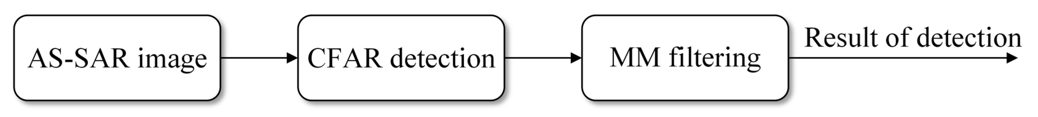
There are many types of FOD on the runway, such as a piece of asphalt concrete or cement concrete, a wrench, a twisted metal strip or the fuel tank cap, and so on, and more of them are small in size and weak in electromagnetic scattering. Moreover, people, vehicles, and aircraft on runways may form strong scattering areas in the images, affecting the target detection performance. The classical detection process of SAR images is shown in Figure 3, which mainly includes constant false alarm rate (CFAR) detection and mathematical morphology (MM) filtering [40,41]. CFAR detector involves a kind of algorithm that uses the difference between the target grayscale and its surrounding neighborhood grayscale for separation, which is widely used for SAR target detection. As a local detection algorithm, the thresholds of the CFAR detector are determined adaptively. The process of MM filtering is used to remove clutter with large differences in size and element targets. In general, through the selection of the size and shape of structural elements, morphological filtering first corrodes the image to remove the small clutter whose size does not meet the element target and then expands the image to maintain the element target in the image. To remove large-scale clutter in the scene, morphological filtering also adopts a similar method to remove small clutter. First, the image with the target removed is obtained, and then the image with the large-scale clutter removed can be obtained by subtracting the image from the original image. After that, target classification can even be realized by feature extraction for detection results [42,43,44].

According to the actual situation of FOD detection, false alarms are the main challenge of classical detection algorithms owing to the lower SNR. AS-SAR can monitor airport runways and other areas for a long time and form sequence of images. Multi-image coherent accumulation is introduced to improve the target SNR and reduce false alarms while ensuring the detection rate. The practical detection flow is given in Figure 4. The effectiveness of this flow depends on the stability of the target phase, so SPD correction is required. At the same time, the stable phase is also an important feature of the target distinguishing background.

3. The Correction Approach to SPD

SPD is caused by atmospheric disturbance and system noise. It has both two-dimensional space-varying and time-varying characteristics. There are always some points with fixed positions in the actual scene, with high SNR and stable scattering characteristics. According to the derivation of the imaging model, the phase change of these scattering points is mainly caused by SPD. Therefore, these scattering points can be used to estimate SPD and called stable phase control points (SPCP) in this paper. This section introduces an adaptively SPD correction approach based on the SPCP, which mainly includes three parts. First, a spatial and temporal model of SPD is established, and the corresponding SPD estimation method is given. Second, the screening method of the SPCP is shown, which is used to estimate the SPD. Third, the complete process flow of the correction approach is obtained.

3.1. Modeling and Estimation of SPD

Setting the values of the monitoring target in two sequential images as ${\alpha }_1{e}^{j{\phi }_1}$ and ${\alpha }_2{e}^{j{\phi }_2}$, SPD Δφ can be calculated by the following equation:

$$\Delta \phi =angle\left({\alpha }_2{e}^{j{\phi }_2}\times {\left({\alpha }_1{e}^{j{\phi }_1}\right)}^{*}\right),$$

(11)

where angle(∙) represents the calculated phase angle and * represents the complex conjugate. Considering that SPD is caused by the system itself and the atmosphere, Δφ can be

$$\Delta \phi =\Delta {\phi }_s+\Delta {\phi }_a+\Delta {\phi }_n,$$

(12)

where $\Delta {\phi }_s$ represents the phase caused by the system itself, Δφ_a represents the phase caused by the atmosphere, and Δφ_n is the noise phase. In general, Δφ_s is constant. The temperature and humidity of the atmosphere change in space over time, which causes the nonuniformity of electromagnetic characteristics, so that the propagation speed and direction of the signal change continuously when passing through the atmosphere. When the atmospheric changes along the range and azimuth are independent of each other, the first-order function model of SPD along the distance and azimuth is established [37,38]:

$$\Delta \phi =\frac{4\pi }{\lambda }\left({\beta }_0+{\beta }_1{r}_g+{\beta }_2{\phi }_g\right)+\Delta {\phi }_n,$$

(13)

where λ is the carrier frequency wavelength, r_g is the ground range from target to radar, and φ_g is the angle between the target and the initial scanning direction of the radar. β₀, β₁, and β₂ are weighting coefficients.

Equation (13) shows that as long as three stable strong scattering points with high SNR are found, the simultaneous equation can be established through their phase drift, and the weighting coefficient can be solved. Here, a stable strong scattering point was described as the SPCP. In fact, the number of SPCPs is much greater than 3. Therefore, the least squares (LS) method will be used to estimate the weighting coefficient. Let $\stackrel{\rightharpoonup }{\beta }=\left[{\beta }_0,{\beta }_1,{\beta }_2\right]$. Equation (13) can be expressed as a matrix as follows:

$$\Delta \phi =\frac{4\pi }{\lambda }\left[1 r_g {\phi }_g\right]\left[\begin{array}{c}{\beta }_0\\ {\beta }_1\\ {\beta }_2\end{array}\right]+e=\stackrel{\rightharpoonup }{h}{\stackrel{\rightharpoonup }{\beta }}^T+e,$$

(14)

where e is the noise matrix, and

$$\stackrel{\rightharpoonup }{h}=\frac{4\pi }{\lambda }\left[1 r_g {\phi }_g\right],$$

(15)

For multiple SPCPs, the matrix is expressed as an equation

$$H=\left[\begin{array}{c}{\stackrel{\rightharpoonup }{h}}_1\\ {\stackrel{\rightharpoonup }{h}}_2\\ ⋮\end{array}\right],\Delta \mathrm{\Phi }=\left[\begin{array}{c}\Delta {\phi }_1\\ \Delta {\phi }_2\\ ⋮\end{array}\right],$$

(16)

The LS algorithm can be used, and

$$\widehat{\stackrel{\rightharpoonup }{\beta }}={\left(H^{T}H\right)}^{-1}{H}^T\Delta \Phi ,$$

(17)

Then, $\widehat{\Delta \phi }$ is estimated as follows:

$$\widehat{\Delta \phi }=\stackrel{\rightharpoonup }{h}{\widehat{\stackrel{\rightharpoonup }{\beta }}}^T,$$

(18)

Due to the time continuity of temperature and humidity changes causing SPD, the estimated SPD can be filtered by a Kalman filter. The state transition matrix can be established, such as the equation:

$$\Delta {\phi }^k=F_1\Delta {\phi }^{k-1}+q_{k-1},$$

(19)

where q_k−1 is Gaussian noise and F₁ is the state transfer matrix. The observation equation is established as follows:

$$z_k=F_2\Delta {\phi }^{k-1}+v_{k-1},$$

(20)

According to actual, the standard deviation of SPD change caused by noise shall not exceed 2 degrees, so the variance matrix Q corresponding to q is set to 4. Considering that the error of SPCPs’ SPD measured by AS-SAR is better than 3 degrees when processing two adjacent frames of images, so the variance matrix V corresponding to v is set to 9. In addition, it is assumed that SPD changes slowly with temperature and humidity, and the observed value is SPD, so F₁ = 1 and F₂ = 1. Then, time-domain filtering of the SPCP can be realized.

3.2. The Screening Method of the SPCP

In the process of SPD calculation, the selection of the SPCP is very important. For amplitude images, three features to screen SPCPs are defined: local image contrast F_l, amplitude dispersion F_d, and correlation coefficient F_c. The screening process flow of the SPCP is shown in Figure 5.

Let the sequence of images be X_n, 1 ≤ n ≤ N, where N is the number of images. x_n(i, j) represents the image X_n amplitude value at pixel point (i, j). Then, F_l, F_d, and F_c are defined as follows:

For F_l, this paper first acquires the neighborhood image slice I_i of each pixel x_n(i, j) in X_n and calculate the mean value $m_b^n\left(i,j\right)$ and standard deviation ${\sigma }_b^n\left(i,j\right)$, then

$$F_l=\frac{1}{N}{{\displaystyle \sum }}_{n=1}^N\frac{x_n\left(i,j\right)-m_b^n\left(i,j\right)}{{\sigma }_b^n\left(i,j\right)},$$

(21)

The larger F_l is, the larger the SNR and the more stable the corresponding pixel.

For F_d, the amplitude mean value m(i, j) and standard deviation σ(i, j) of each pixel x_n(i, j) in the sequence of images are calculated, and then it is calculated by

$$F_d=\frac{m\left(i,j\right)}{\sigma \left(i,j\right)},$$

(22)

The larger F_d is, the more stable the amplitude information is. Given that the calculation of F_d only uses the amplitude information, it has the advantages of a small amount of calculation and easy extraction.

For F_c, the correlation coefficient of each pixel of the sequence of images needs to be calculated according to the following equation:

$$c_{n-1}\left(i,j\right)=\frac{\left|{{\displaystyle \sum }}_{i=1}^I{{\displaystyle \sum }}_{j=1}^J{x}_n\left(i,j\right)x_{n-1}\left(i,j\right)\right|}{\sqrt{{{\displaystyle \sum }}_{i=1}^I{{\displaystyle \sum }}_{j=1}^J{\left|x_n\left(i,j\right)\right|}^2{{\displaystyle \sum }}_{i=1}^I{{\displaystyle \sum }}_{j=1}^J{\left|x_{n-1}\left(i,j\right)\right|}^2}},$$

(23)

where I and J are sliding neighborhood window sizes. Then, the mean m_c(i, j) of each c_n(i, j) is calculated, and F_c is acquired by

$$F_c=m_c\left(i,j\right),$$

(24)

The larger F_c is, the stronger the correlation. F_c involves the neighborhood of pixels, which has a large amount of calculation, but the feature is stable and less disturbed by noise.

Each extracted feature is formed into a vector, $\stackrel{\rightharpoonup }{F}=\left[F_l,F_d,F_c\right]$. Considering that the values of each component of the feature vector are not uniform and have different effects on the linear classifier, it is necessary to normalize it. According to the principle of Mahalanobis distance measurement [45], this paper solves the problem of different dimension distribution through covariance normalization. Covariance matrix ${\mathrm{\Sigma }}_{\stackrel{\rightharpoonup }{F}}$ can be obtained by

$$C=\left(\stackrel{\rightharpoonup }{F}-{\mu }_{\stackrel{\rightharpoonup }{F}}\right){\left(\stackrel{\rightharpoonup }{F}-{\mu }_{\stackrel{\rightharpoonup }{F}}\right)}^T=U^T{\mathrm{\Sigma }}_{\stackrel{\rightharpoonup }{F}}U,$$

(25)

where U is the unitary matrix, ${\mu }_{\stackrel{\rightharpoonup }{F}}$ is the mean value of feature vectors, and T is the transpose operation. Then, the normalized feature vector ${\stackrel{\rightharpoonup }{F}}_u$ can be represented by the following equation:

$${\stackrel{\rightharpoonup }{F}}_u=\left(\stackrel{\rightharpoonup }{F}-{\mu }_{\stackrel{\rightharpoonup }{F}}\right){\mathrm{\Sigma }}_{\stackrel{\rightharpoonup }{F}}^{-1},$$

(26)

In the process of classification, a linear classification decision criterion is established:

$$h({\stackrel{\rightharpoonup }{F}}_u)=W^T{\stackrel{\rightharpoonup }{F}}_u+{\omega }_0,$$

(27)

where W^T and ω₀ are weighting coefficients, which can be obtained through known calibration target training. In the training process, to ensure the computational efficiency and the expansibility of the approach, the number of SPCPs in this paper is limited to 0.5–1% of the total number of image points. Then, on this basis, the training obtains the weighting coefficients when the number of SPCPs falling in fixed areas such as guardrails and buildings accounts for the highest number of total SPCPs. At the same time, the robustness and consistency of radar performance are good and the SNR meets the monitoring conditions; the classification process has expansibility.

3.3. The Process Flow of Correction Approach

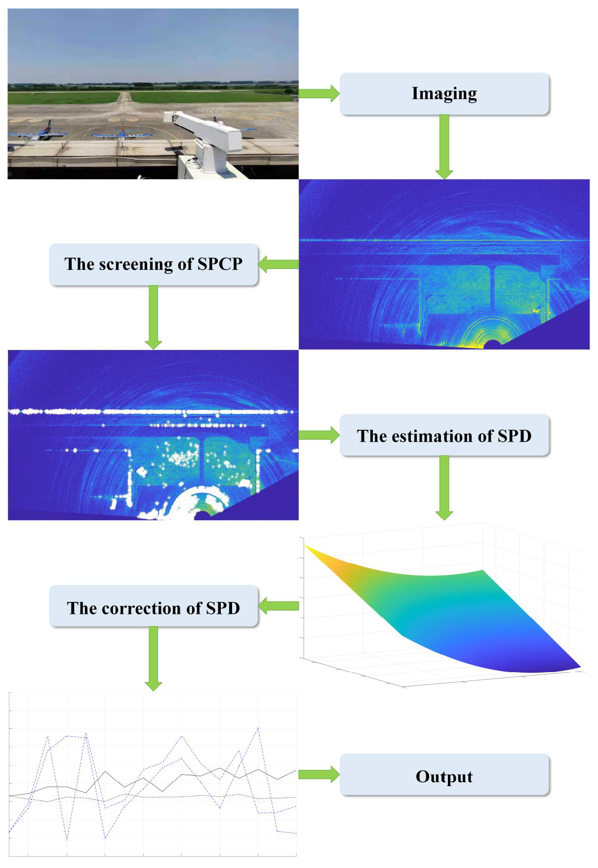
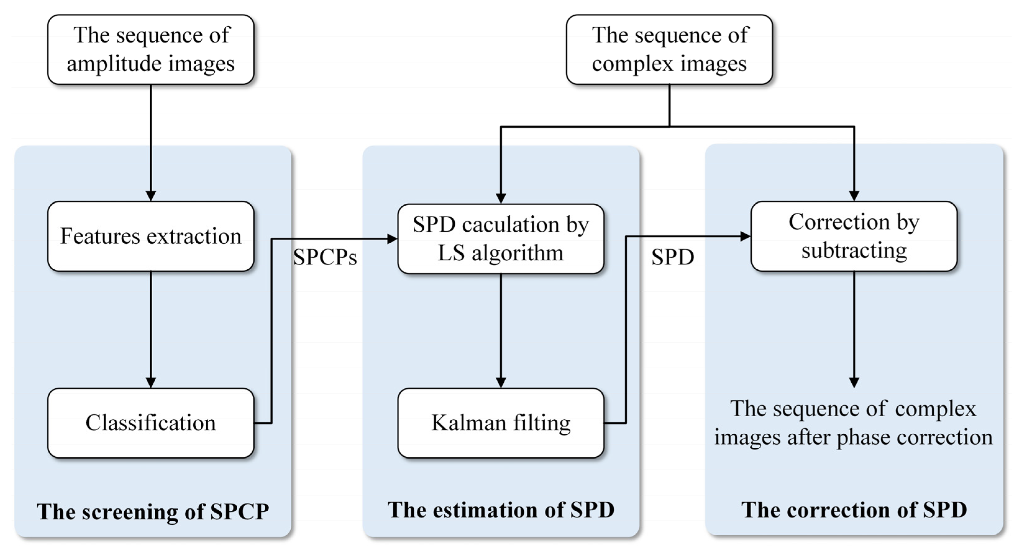
Figure 6 shows the complete process flow of the correction approach. It consists of three stages:

• The screening of the SPCP. This stage can be completed in real time or offline. To prevent the FOD target from being used as an SPCP, it needs empty scene data. It processes the sequence of amplitude images through feature extraction and classification and sends the obtained SPCPs to the second stage.
• The estimation of the SPD. In the actual processing process, using the SPCPs provided in the first stage and based on the SPD model, the SPD between two complex images is estimated in real time by the LS algorithm. Finally, the Kalman filter is carried out based on the multiframe SPD (greater than 2) to obtain the SPD for correction.
• The correction of the SPD. Expected correction is achieved by subtracting the SPD, and the sequence of complex images after phase correction are produced and output.

4. Results

To demonstrate the effectiveness of the proposed correction approach to SPD, the experimental results based on the measured AS-SAR data are presented. Figure 7 shows the AS-SAR and its working field scene, and the corresponding image is shown in Figure 8. The 16-bit sampling data of radar echo is processed directly using the imaging process shown in Figure 2 to obtain the image $s_I$. Considering the large value of s_I amplitude, which is not conducted to display. Therefore, Figure 8 and subsequent AS-SAR images are obtained using the function 20 × log₁₀(s_I). Thus, AS-SAR is able to effectively image the monitored area on the runway. As described above, the screening of SPCPs is very important. These points are extracted according to Section 3.2, as shown in Figure 9. Compared with the actual scene, the selected SPCPs are mainly fixed targets such as fences and houses. It can be assumed that their phase change is independent of the position change and is mainly caused by SPD. Thus, they can be used to estimate the whole scene SPD.

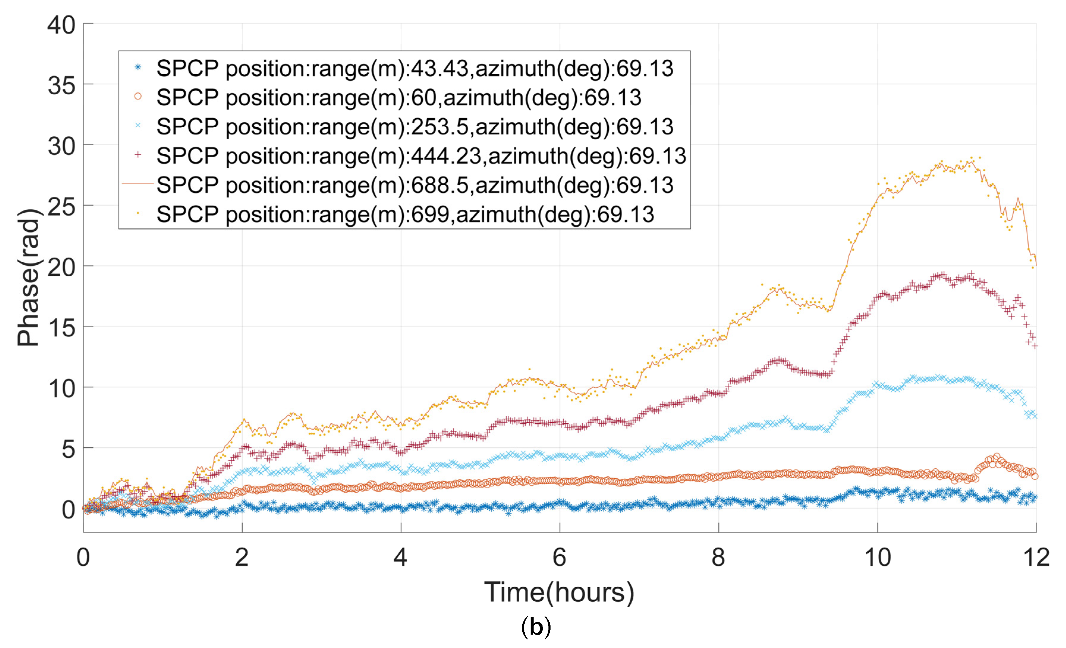
To estimate the SPD more accurately, it is necessary to analyze the phase change history of SPCPs, as shown in Figure 10. All initial phases are aligned to 0, and the duration of continuous monitoring is 12 h. Figure 10a shows the phase change history of SPCPs with the same range and different azimuths. The phase difference between them is small. Figure 10b shows the phase change history of SPCPs with different ranges and the same azimuth. The farther they are from the radar, the greater the phase change.

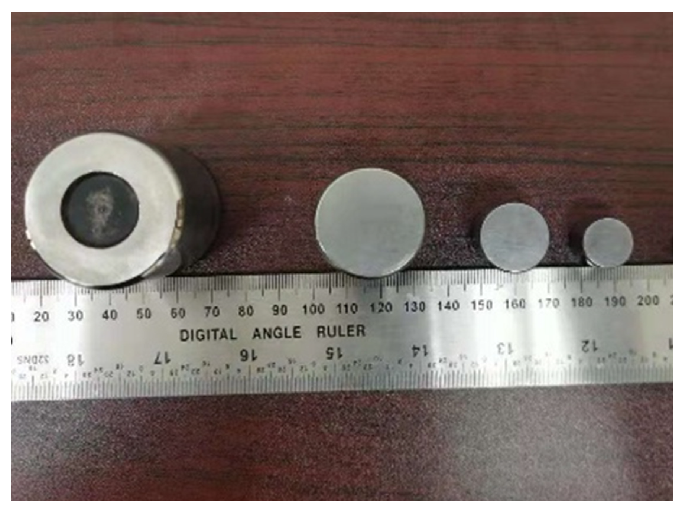
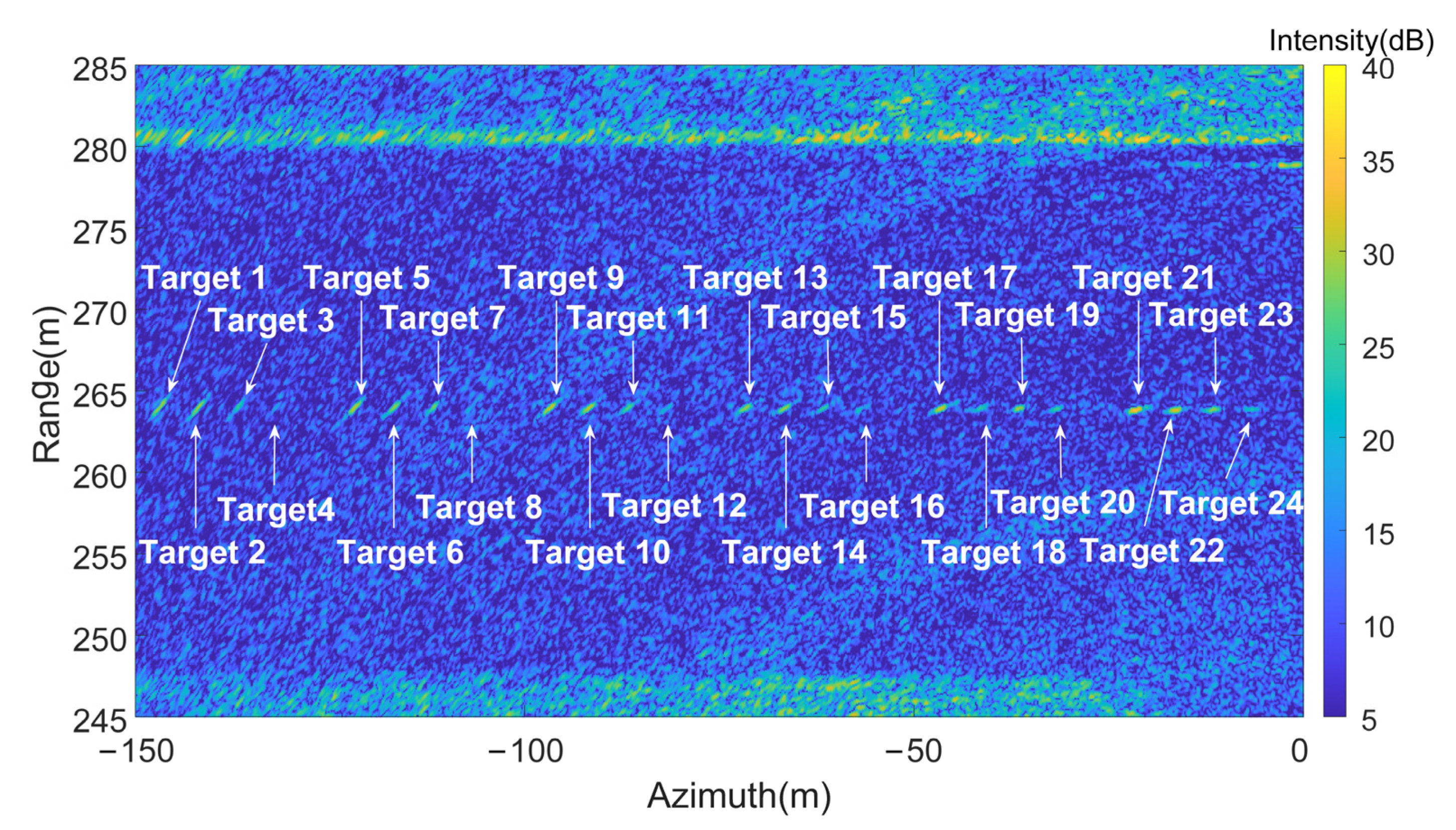
In this paper, the cylindrical targets shown in Figure 11 are analyzed, and their height and diameter are equal. The target is arranged on the runway, as shown in Figure 12, and

Table 1. Correspondence table between cylinder size and target number.

ID	Cylinder Size(cm)		Target Number
	Height	Diameter
1	4	4	target 1, target 5, target 9, target 13, target 17, target 21
2	3	3	target 2, target 6, target 10, target 14, target 18, target 22
3	2	2	target 3, target 7, target 11, target 15, target 19, target 23
4	1.5	1.5	target 4, target 8, target 12, target 16, target 20, target 24

gives correspondence between cylinder size and target number.

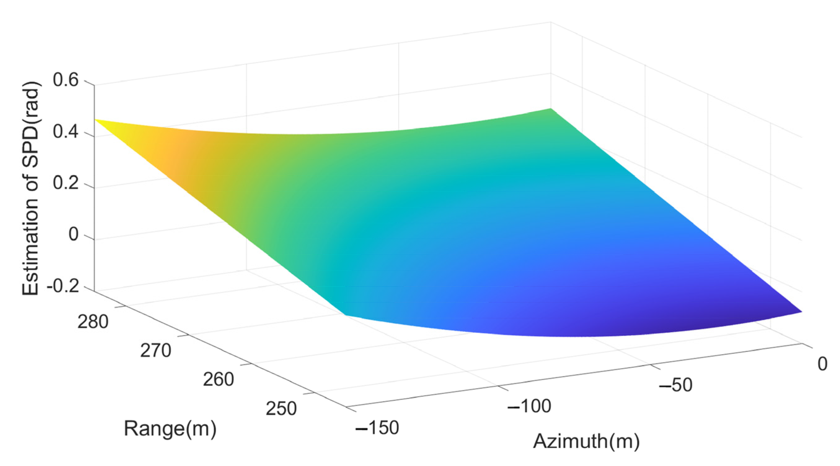
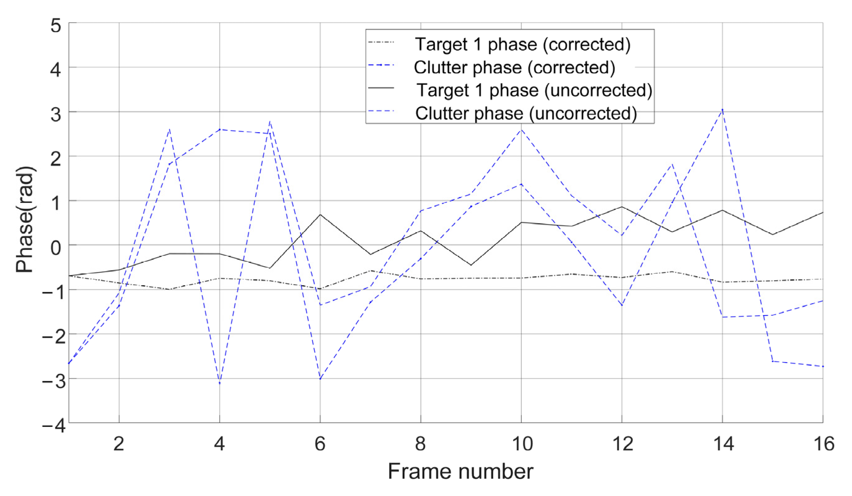
In the actual experimental process, the SPD is estimated using the LS algorithm and Kalman filter. Figure 13 gives an estimated SPD image of two AS-SAR images. Consistent with the actual measurement results, SPD is more affected by range. Then, a correction is achieved by subtracting the SPD. Figure 14 shows the phase change history of target 1 and clutter. Through comparison, it is found that the target phase changes more than 1.2 rad after 16 frames before the correction, while the target phase changes less than 0.5 when the SPD is corrected. Moreover, the phase change history of clutter is random. The correction approach proposed in this paper can effectively maintain the stability of the target phase. In addition, the stable phase can also be used to distinguish the target from the background.

5. Discussion

According to Section 2.2, false alarms are the main challenge of classical detection algorithms owing to the lower SNR. Coherent accumulation is needed in the FOD detection process to improve the SNR. The stable phase guarantees improved coherent accumulation performance. Figure 15 shows a comparison of coherent accumulation images. Compared with the original single image, the background noise in the scene is reduced after coherent accumulation. When more images are accumulated, the better the SNRs are. At the same time, the accumulation effect of the SPD correction is better than that of no correction.

The quantitative analysis results are shown in Figure 16 and

Table 2. The SNR of targets (dB).

Number of Targets	The Number of Coherent Accumulation Images
	1	Before Correction			After Correction
		4	8	16	4	8	16
Target 1	12.33	19.47	24.58	32.66	20.51	28.85	34.05
Target 2	13.12	22.97	28.82	31.20	23.95	28.81	32.13
Target 3	6.84	26.19	24.83	29.36	26.30	23.61	27.99
Target 4	3.49	11.83	20.84	25.70	13.80	21.80	25.43
Target 5	9.37	28.38	36.33	37.72	30.95	34.35	38.69
Target 6	13.40	26.76	31.72	36.12	26.67	33.32	37.75
Target 7	4.60	22.18	20.67	27.81	21.51	23.68	31.67
Target 8	0.73	9.99	15.08	25.49	10.78	16.80	27.96
Target 9	16.99	18.27	26.24	25.99	20.42	28.31	27.03
Target 10	8.88	15.36	23.30	30.11	16.77	24.10	30.86
Target 11	13.45	18.52	24.46	29.26	18.43	25.07	29.77
Target 12	4.94	16.58	26.45	30.21	16.21	26.07	33.06
Target 13	8.90	19.76	26.65	32.00	19.78	26.22	31.91
Target 14	8.53	19.39	23.02	26.53	18.51	23.91	26.59
Target 15	7.30	21.40	25.02	31.92	25.35	27.84	33.45
Target 16	−5.68	14.20	17.72	24.69	15.86	20.68	26.25
Target 17	13.66	25.98	28.85	38.49	26.45	28.68	36.85
Target 18	1.59	18.23	26.12	28.98	18.79	27.61	30.98
Target 19	8.09	23.74	38.20	46.31	22.05	36.60	47.04
Target 20	2.12	10.90	18.27	21.93	12.52	18.13	23.37
Target 21	16.79	34.53	37.00	38.55	35.05	37.86	39.27
Target 22	13.34	31.24	40.71	43.50	33.26	42.48	44.30
Target 23	12.89	21.95	31.24	37.11	22.52	30.04	37.98
Target 24	6.77	18.60	21.21	30.12	21.40	23.80	30.35

. Figure 16 gives a comparison of target SNRs between uncorrected and corrected samples. Figure 16a shows the comparison of the target SNR after coherent accumulation using 4 images. The actual value curve of the target SNR, which is corrected, is mostly above its uncorrected value. Their corresponding mean values of the target SNRs are 20.68 dB and 21.58 dB, and the effect of coherent accumulation is better after correction. When the number of accumulated images becomes 8 and 16, it shows similar characteristics, as shown in Figure 16b,c. For coherent accumulation using 8 images, the corresponding mean values are 26.56 dB and 27.44 dB. For coherent accumulation using 16 images, the corresponding mean values are 31.74 dB and 32.70 dB. At the same time, when 4 images, 8 images, and 16 images are coherently accumulated, their maximum SNR demonstrates increases of 3.95 dB, 4.27 dB, and 3.86 dB, respectively. Table 2 gives the SNR results of 24 targets under different conditions, while the values with better SNRs are bold. Coherent accumulation can effectively improve the target SNR. Moreover, after SPD correction, the SNR of most targets improved significantly. Therefore, this approach makes the phase stability of the same target in multi-frame images better and proves the effectiveness of SPD correction from the side.

6. Conclusions

In this paper, maintaining the stability of the target phase is the key to coherent accumulation in FOD detection flow. Through the analysis of the AS-SAR imaging model, it is concluded that the theoretical phase of the target is only related to its position, and its change is the SPD, which is mainly caused by atmospheric disturbances and system hardware. Based on SPD modeling, a complete process flow of the correction approach is proposed. It adaptively screens SPCPs through the normalized features of local image contrast, amplitude dispersion, and core translation coefficient, and then makes full use of spatial filtering and temporal filtering to ensure the accuracy of correction. The real data results show that the SNR of most targets after the correction has improved significantly. Therefore, this approach makes the phase stability of the same target in multi-frame images better, which indirectly proves the effectiveness of SPD correction. However, the approach in this paper also has some shortcomings. First, the time model is relatively simple and does not introduce the relevant information of temperature and humidity changes. Second, the number of SPCPs screened is large, which affects the calculation efficiency. At the same time, the number of SPCPs at the edge of the runway is relatively small, which will also affect the spatial filtering effect of SPD. Therefore, it is necessary to further study and improve the spatial and temporal model of SPD.

References

- Marandi, S.M.; Rahmani, K.; Tajdari, M. Foreign object damage on the leading edge of gas turbine blades. Aerosp. Sci. Technol. 2014, 33, 65–75. [Google Scholar] [CrossRef]
- ICAO. Proposals for amendment to pans-aerodromes (DOC 9981). In Proceedings of the third meeting of the aerodromes operations and planning-Working Group (AOP/WG/3), Bangkok, Thailand, 24–26 June 2019; Available online: https://www.icao.int/APAC/Meetings/Pages/2019-AOP-SG3-GRF-Seminar.aspx (accessed on 20 October 2021).
- Patterson, J. Foreign Object Debris (FOD) Detection Research. Int. Airpt. Rev. 2008, 11, 22–26. [Google Scholar]
- Woodworth, E. Procedures for FOD Detection System Performance Assessments: Radar-Based and Dual Sensor Systems. In Proceedings of the 2010 FAA Worldwide Airport Technology Transfer Conference, Atlantic City, NJ, USA, 20–22 April 2010. [Google Scholar]
- Lazar, P.; Herricks, E.E. Procedures for FOD Detection System Performance Assessments: Electro-Optical FOD Detection System. In Proceedings of the FAA Worldwide AirportTechnology Transfer Conference, Atlantic City, NJ, USA, 20–22 April 2010. [Google Scholar]
- Shelley, P.H.; Vahey, P.G.; Werner, G.J.; Kisch, R.A. Multispectral Imaging System and Method for Detecting Foreign Object Debris. US Patent 14/552,697, 25 November 2014. [Google Scholar]
- Herricks, E.E.; Woodworth, E.; Patterson, J., Jr. Performance Assessment of a Hybrid Radar and Electro-Optical Foreign Object Debris Detection System. DOT/FAA/TC-12/22. U.S. Department of Transportation Federal Aviation Administration. 2012; pp. 1–46. Available online: https://www.tc.faa.gov/its/worldpac/techrpt/tc12-22.pdf (accessed on 20 October 2021).
- Leonard, T.; Lamont-Smith, T.; Hodges, R.; Beasley, P. 94-GHz Tarsier radar measurements of wind waves and small targets. In European Microwave Week 2011: Wave to the Future, EuMW 2011, Proceedings of the 8th European Radar Conference, EuRAD, Manchester, UK, 12–14 October 2011; IEEE: Piscataway, NJ, USA; pp. 73–76. Available online: https://ieeexplore.ieee.org/document/6100969 (accessed on 20 October 2021).
- Trex Aviation Systems. FOD Finder. 2021. Available online: www.fodfinder.com/index.html (accessed on 20 October 2021).
- Xsight Systems. FODetect Installation Manual. 2021. Available online: www.xsightsys.com (accessed on 20 October 2021).
- Feil, P.; Menzel, W.; Nguyen, T.P.; Pichot, C.; Migliaccio, C. Foreign objects debris detection (FOD) on airport runways using a broadband 78 GHz sensor. In Proceedings of the 2008 European Radar Conference, Amsterdam, The Netherlands, 30–31 October 2008; pp. 451–454. [Google Scholar] [CrossRef]
- Wu, J. Echo Modeling of Radar for Foreign Objects Debris Detection on Airport Runways. J. Terahertz Sci. Electron. Inf. Technol. 2013, 11, 917–921. [Google Scholar]
- Yu, I.; Xiao, G. Study and design on FOD detection and surveillance system for airport runway. Laser Infrared 2011, 41, 909–915. [Google Scholar]
- Liu, S.Q.; Hu, S.H.; Xiao, Y.; Zhao, J.; Liu, X.L. Airport runway radar image de-noising based on 2-D shift-invariance hybrid transform. Syst. Eng. Electron. 2015, 37, 73–78. [Google Scholar]
- Cao, T.T. The Build of Airport Runway Fod Detection System and Algorithm Study Based on Radar Image. Master’s Thesis, Beijing Jiaotong University, Beijing, China, 2012. [Google Scholar]
- Curlander, J.C.; McDonough, R.N. Synthetic Aperture Radar: Systems and Signal Processing; Wiley: New York, NY, USA, 1991. [Google Scholar]
- Huang, Z.; Pan, Z.; Lei, B. Transfer Learning with Deep Convolutional Neural Network for SAR Target Classification with Limited Labeled Data. Remote Sens. 2017, 9, 907. [Google Scholar] [CrossRef] [Green Version]
- Wang, Y.; Wang, C.; Zhang, H.; Dong, Y.; Wei, S. A SAR Dataset of Ship Detection for Deep Learning under Complex Backgrounds. Remote Sens. 2019, 11, 765. [Google Scholar] [CrossRef] [Green Version]
- Bianchini Ciampoli, L.; Gagliardi, V.; Ferrante, C.; Calvi, A.; D’Amico, F.; Tosti, F. Displacement Monitoring in Airport Runways by Persistent Scatterers SAR Interferometry. Remote Sens. 2020, 12, 3564. [Google Scholar] [CrossRef]
- Lort, M.; Aguasca, A.; López-Martínez, C.; Fabregas, X. Impact of Wind-Induced Scatterers Motion on GB-SAR Imaging. IEEE J. Sel. Top. Appl. Earth Obs. Remote Sens. 2018, 11, 3757–3768. [Google Scholar] [CrossRef] [Green Version]
- Aguasca, A.; Broquetas, A.; Fábregas, X.; Mallorqui, J.J.; Vilalvilla, P.; Biscamps, J.; Llop, J.; Gallart, M.; Gil, E.; Gras, A. Hydrosoil, Soil Moisture and Vegetation Parameters Retrieval with a C-Band GB-SAR: Campaign Implementation and First Results. In Proceedings of the 2021 IEEE International Geoscience and Remote Sensing Symposium IGARSS, Brussels, Belgium, 17–22 July 2021; pp. 6685–6687. [Google Scholar] [CrossRef]
- Andre, D.; Morrison, K.; Blacknell, D.; Muff, D.; Nottingham, M.; Stevenson, C. Very high resolution Coherent Change Detection. In Proceedings of the 2015 IEEE Radar Conference (RadarCon), Arlington, VA, USA, 27–30 October 2015; pp. 0634–0639. [Google Scholar] [CrossRef]
- André, D.; Blacknell, D.; Morrison, K. Spatially variant incoherence trimming for improved bistatic SAR CCD. In Proceedings of the 2013 IEEE Radar Conference (RadarCon13), Ottawa, ON, Canada, 29 April–3 May 2013; pp. 1–6. [Google Scholar] [CrossRef]
- Roedelsperger, S.; Laeufer, G.; Gerstenecker, C.; Becker, M. Monitoring of displacements with ground-based microwave interferometry: IBIS-S and IBIS-L. J. Appl. Geod. 2010, 4, 41–54. [Google Scholar] [CrossRef]
- Federal Aviation Administration. Airport Engineering, Design, & Construction—Airports. 2022. Available online: https://www.faa.gov/airports/engineering/ (accessed on 20 February 2022).
- Civil Aviation Administration of China. Regulations on the Administration of Special Equipment for Civil Airports. CCAR-137CA-R4. 2022. Available online: http://www.caac.gov.cn/XXGK/XXGK/MHGZ/201706/t20170612_44707.html (accessed on 20 February 2022).
- Klausing, H. Feasibility of a synthetic aperture radar with rotating antennas (ROSAR). In Proceedings of the Ninth European Microwave Conf., London, UK, 4–7 September 1989; pp. 287–299. [Google Scholar]
- Lee, H.; Lee, J.H.; Kim, K.E.; Sung, N.H.; Cho, S.J. Development of a Truck-Mounted Arc-Scanning Synthetic Aperture Radar. IEEE Trans. Geosci. Remote Sens. 2014, 52, 2773–2779. [Google Scholar] [CrossRef]
- Wang, Y.; Song, Y.; Lin, Y.; Li, Y.; Zhang, Y.; Hong, W. Interferometric DEM-Assisted High Precision Imaging Method for ArcSAR. Sensors 2019, 19, 2921. [Google Scholar] [CrossRef] [PubMed] [Green Version]
- Takenaka, H.; Sakashita, T.; Higuchi, A.; Nakajima, T. Geolocation Correction for Geostationary Satellite Observations by a Phase-Only Correlation Method Using a Visible Channel. Remote Sens. 2020, 12, 2472. [Google Scholar] [CrossRef]
- Zebker, H. Accuracy of a Model-Free Algorithm for Temporal InSAR Tropospheric Correction. Remote Sens. 2021, 13, 409. [Google Scholar] [CrossRef]
- Hu, Z.; Mallorquí, J.J. An Accurate Method to Correct Atmospheric Phase Delay for InSAR with the ERA5 Global Atmospheric Model. Remote Sens. 2019, 11, 1969. [Google Scholar] [CrossRef] [Green Version]
- Qin, F.; Bu, X.; Liu, Y.; Liang, X.; Xin, J. Foreign Object Debris Automatic Target Detection for Millimeter-Wave Surveillance Radar. Sensors 2021, 21, 3853. [Google Scholar] [CrossRef]
- Wan, Y.; Liang, X.; Bu, X.; Liu, Y. FOD Detection Method Based on an Iterative Adaptive Approach for Millimeter-Wave Radar. Sensors 2021, 21, 1241. [Google Scholar] [CrossRef]
- Iannini, L.; Guarnieri, A.M. Atmospheric Phase Screen in Ground-Based Radar: Statistics and Compensation. IEEE Geosci. Remote Sens. Lett. 2011, 8, 537–541. [Google Scholar] [CrossRef]
- Dong, J.; Dong, Y. Atmospheric artifact compensation for deformation monitoring with ground-based radar. Eng. Surv. Mapp. 2014, 23, 72–75. [Google Scholar] [CrossRef]
- Deng, Y.; Hu, C.; Tian, W.; Zhao, Z. A Grid Partition Method for Atmospheric Phase Compensation in GB-SAR. IEEE Trans. Geosci. Remote Sens. 2022, 60, 1–13. [Google Scholar] [CrossRef]
- Noferini, L.; Pieraccini, M.; Mecatti, D.; Luzi, G.; Atzeni, C.; Tamburini, A.; Broccolato, M. Permanent Scatterers Analysis for Atmospheric Correction in Ground Based SAR Interferometry. IEEE Trans. Geosci. Remote Sens. 2005, 43, 1459–1471. [Google Scholar] [CrossRef]
- Luo, Y.; Song, H.; Wang, R.; Deng, Y.; Zhao, F.; Xu, Z. Arc FMCW SAR and Applications in Ground Monitoring. IEEE Trans. Geosci. Remote Sens. 2014, 52, 5989–5998. [Google Scholar] [CrossRef]
- Liu, W.; Zhang, Z.; Yu, X. FOD Detection on Airport Runway with an Adaptive CFAR Technique. In International Conference on Communications Signal Processing and Systems Lecture Notes in Electrical Engineering; Springer: Berlin/Heidelberg, Germany, 2014; Volume 246, pp. 637–645. [Google Scholar]
- Izzo, A.; Liguori, M.; Clemente, C.; Galdi, C.; Di Bisceglie, M.; Soraghan, J.J. Multimodel CFAR Detection in Foliage Penetrating SAR Images. IEEE Trans. Aerosp. Electron. Syst. 2017, 53, 1769–1780. [Google Scholar] [CrossRef] [Green Version]
- Dai, J.H.; Chen, J.L. Feature selection via normative fuzzy information weight with application into tumor classification. Appl. Soft Comput. 2020, 92, 106299. [Google Scholar] [CrossRef]
- Dai, J.H.; Hu, H.; Wu, W.Z.; Qian, Y.H.; Huang, D.B. Maximal Discernibility Pairs based Approach to Attribute Reduction in Fuzzy Rough Sets. IEEE Trans. Fuzzy Syst. 2018, 26, 2174–2187. [Google Scholar] [CrossRef]
- Jin, T.; Zhou, Z.M.; Song, Q.; Chang, W.G. The evidence framework applied to fuzzy hypersphere SVM for UWB SAR landmine detection. ICSP2006 Proc. 2006, 3, 1–4. [Google Scholar]
- Webb, A.R. Statistical Pattern Recognition, 3rd ed.; John Wiley & Sons Ltd.: Chichester, UK, 2002; pp. 167, 310, 360, 427. [Google Scholar]
Figure 1.
Geometric model of AS-SAR.
Figure 2.
Imaging flow of the radar.
Figure 3.
The classical detection flow of SAR images.
Figure 4.
The practical detection flow of SAR images.
Figure 5.
Screening process flow of the SPCP.
Figure 6.
The complete process flow of the correction approach.
Figure 7.
AS-SAR and its working field scene.
Figure 8.
AS-SAR image of the runway.
Figure 9.
The screening results of SPCPs.
Figure 10.
The phase change history of SPCPs: (a) with the same range and different azimuths; (b) with different ranges and the same azimuth.
Figure 11.
The photo of cylindrical targets.
Figure 12.
Layout diagram of cylindrical targets on the runway.
Figure 13.
Estimated SPD between two AS-SAR images.
Figure 14.
The phase change history of two targets.
Figure 15.
The comparison of coherent accumulation images: (a) using 4 images (uncorrected); (b) using 4 images (corrected). (c) using 8 images (uncorrected); (d) using 8 images (corrected). (e) using 16 images (uncorrected); (f) using 16 images (corrected).
Figure 16.
The comparison of target SNRs between uncorrected and corrected samples: (a) using 4 images; (b) using 8 images; (c) using 16 images.