Estimation of Building Thermal Performance using Simple Sensors and Air Conditioners


1
Graduate School of Science and Technology, Keio University, 3-14-1 Hiyoshi, Kohoku, Yokohama, Kanagawa 223-8522, Japan
2
Department of System Design Engineering, Faculty of Science and Technology, Keio University, 3-14-1 Hiyoshi, Kohoku, Yokohama, Kanagawa 223-8522, Japan
*
Author to whom correspondence should be addressed.
Energies 2019, 12(15), 2950; https://doi.org/10.3390/en12152950
Submission received: 9 June 2019
/
Revised: 7 July 2019
/
Accepted: 29 July 2019
/
Published: 31 July 2019
(This article belongs to the Special Issue Sustainable Energy Consumption)
Abstract
:Energy and environmental problems have attracted attention worldwide. Energy consumption in residential sectors accounts for a large percentage of total consumption. Several retrofit schemes, which insulate building envelopes to increase energy efficiency, have been adapted to address residential energy problems. However, these schemes often fail to balance the installment cost with savings from the retrofits. To maximize the benefit, selecting houses with low thermal performance by a cost-effective method is inevitable. Therefore, an accurate, low-cost, and undemanding housing assessment method is required. This paper proposes a thermal performance assessment method for residential housing. The proposed method enables assessments under the existing conditions of residential housings and only requires a simple and affordable monitoring system of power meters for an air conditioner (AC), simple sensors (three thermometers at most), a BLE beacon, and smartphone application. The proposed method is evaluated thoroughly by using both simulation and experimental data. Analysis of estimation errors is also conducted. Our method shows that the accuracy achieved with the proposed three-room model is 9.8% (relative error) for the simulation data. Assessments on the experimental data also show that our proposed method achieved Ua value estimations using a low-cost system, satisfying the requirements of housing assessments for retrofits.
1. Introduction
Attention to energy and environmental problems is increasing worldwide. Energy consumption in the residential sector accounts for a large percentage of total energy consumption. For example, households consumed 29% of the total electricity usage in Japan [1]. One solution to address this issue is retrofitting of buildings. Several subsidization schemes for building retrofit have been introduced worldwide, such as the Green New Deal (GND) schemes [2]. In Japan, subsidization plans for insulating building envelopes were introduced in 2018 [3]. One key to the success of these retrofit schemes is finding houses that benefit from participating in the scheme in cost-effective ways. Guaranteeing a balance between the retrofit cost and the savings after the retrofit is important. For example, GND schemes aim to redeem the retrofit cost from the reduction in electricity bills. In GND schemes, governments or investors pay the initial expense of retrofits instead of homeowners. Then, the retrofit expenses are redeemed to payers from the reduced electricity costs resulting from the retrofits. Long-term reduction in electricity costs per year after retrofits is known to be approximately $149 to $212 [4]. Retrofit cost is more expensive than these savings. Introducing double-glazed windows costs about $800 to $1500 in Japan. It is inferred that the retrofit expense should be redeemed from a long-term and certain reduction in electricity costs to balance the initial investment. Therefore, selecting houses that will benefit from the retrofit is important, especially for retrofit schemes such as GND.
To select houses which benefit from retrofits, assessments of building thermal performance are required. Commonly used assessment index is the average transmission heat transfer coefficient of the fabric of the buildings (Ua value). This study focuses on assessing thermal performance using Ua values. In contrast to assessments that use literature values, assessments that use sensor data collected directly from target buildings (i.e., in situ measurements) are preferred. In situ measurements address the problem of performance gap [5,6,7], or the difference between literature values designed before construction and actual performance achieved during use. Additionally, assessments that don’t need construction details, materials, or questionnaires are useful for assessing existing buildings for which construction details are often missing.
In situ measurements are categorized into destructive and non-destructive methods. We focus on non-destructive methods. One non-destructive method utilizes infrared cameras [8,9,10,11]. Tejedor et al. [10] built a measuring system composed of an IR camera, a reflector, and a blackbody and achieved short-time measurements of 2–3 h. Their results show a deviation of 3–4% from literature values. However, the experimental apparatus is relatively expensive and disturbing to residents.
Another category of non-destructive in situ measurements is co-heating test [12,13,14,15]. Co-heating test estimates building thermal performance by calculating net heating energy demand to keep the whole building in constant internal temperature usually under unoccupied conditions. The major drawbacks are the installment cost of experimental apparatus and disturbance to residents. To achieve costless measurements, monitoring systems using relatively low cost environmental and electric sensors are proposed in several studies [16,17]. Another approach is utilizing existing heating systems. Farmer et al. [18] utilizes the housing’s own central heating systems. To alleviate disturbance to residents, approaches to shorten experimental duration are proposed such as quick U-value of buildings (QUB) [19] and ISABELLE (in situ assessment of the building envelope performances) [20]. These methods use thermal models to deal with dynamic indoor conditions. Co-heating test requires to heat the whole house that may increase the energy costs. To cope with this limitation, Yanagisawa et al. [21] expanded the technique to enable assessments in buildings where non-heated rooms exist. They measured the temperature of a heated room (i.e., living room), a non-heated room (i.e., bathroom), and outdoor ambient air under in-use conditions to calculate defined assessment metrics. However, this method still suffers from the limitations that steady states must be achieved. It can be demanding to occupants.
Another approach of in situ measurement is an identification method that studies suitable models to represent complex building thermal physics [22]. Identification methods often use grey-box models that are simplified representation from the understanding of the physics of heat transfers in a building. Some studies use simulation data to select an accurate model [23,24]. To address the complexity of the model and the high computation time, Leeuwen et al. [25] proposed identification methods that use simple grey-box models in consideration of realistic applications such as HVAC control. Further, Andersen et al. [26] achieved a detailed estimation of the thermal performance of walls in a real environment. They further analyzed errors due to solar radiation. However, the proposed methods have the limitation of requiring detailed sensor data, including solar radiation, which increases the installment cost. In addition, the experiments were done in an ideal environment without residents and arctic winter conditions. Kim et al. [27] developed in situ measurement methods under in-use conditions of buildings. They considered the presence of unmeasured disturbance in the model. However, this method uses detailed sensor data that require expensive data collection systems.
In this study, we propose a low-cost and simple building thermal performance assessment technique for occupied houses. This method enables estimation of the Ua value, which is often used as the criteria for building thermal performance in construction laws. Our method uses data directly measured from constructed houses to address the performance gap. The total cost of a data acquisition system is below around $200 at maximum and may be affordable because the savings by retrofits are known to be close to this amount. To achieve a low-cost installment, we assume a costless monitoring system composed of a power meter for an AC and thermometers, BLE beacon, and smartphone application. The electric consumption of the AC and some temperature data can also be retrieved via communication modules of ACs. They are often implemented in modern ACs that several data can be accessed using protocols such as ECHONET Lite [28]. Therefore, our method could even be implemented as a function of ACs that provide future HVAC services. Using existing ACs for assessments is beneficial because thermal performance can be continuously monitored even after the retrofit. Residents and investors can check the effects of the retrofit. In addition, our proposed method is simple and undemanding to residents. We use a simple measurement system with a limited number of sensors. For example, two or three small sensors in a room may not disturb residents. After the measurement system is installed, the collected data can be assessed remotely without disturbing the residents. In summary, the requirements for the proposed methods are the following:
- Accurate
- Low installment cost
- Simple and undemanding to residents
To satisfy these requirements, we made two contributions to this study. First, we proposed the thermal model of buildings using grey-box representations for the estimation of Ua values that enables the assessments using ACs. Second, we developed data selection and preprocessing techniques to achieve an estimation of Ua values under in-use conditions and in consideration of the characteristics of ACs. This research builds on and expands our previous work [29] in the perspective of modeling and error analysis. A thorough evaluation using both simulation and experimental data is done. Analysis of estimation errors is also performed to develop data selection techniques. We present possible factors that may be challenging when our techniques are used as an application of ACs.
2. Methodology
The thermal dynamics of a building is modeled to estimate Ua values. Since this research aims to perform housing assessments for retrofits, the estimation method should reduce the required number of sensors and avoid errors induced by noise. Simplified models with a limited number of terms and variables were used. In addition, data selection and preprocessing techniques were used to avoid noise in data collected from buildings in-use.
2.1. Grey-Box Models
We consider heat exchange models for a typical Japanese two-story detached house, consisting of a living room located on the first floor, whose volume accounts for a large percentage of the whole house, and two or three bedrooms on the second floor, and an air conditioner (AC) is used. For the purpose of reducing the total cost of the system, we consider the heat exchange within the living room that accounts for a large percentage of the total volume of the house.
We assume typical electric refrigerant-based AC units used in Japan. They are air sourced and bivalent. Various sensors are implemented in the ACs. Our proposed method only requires information on the electricity consumption of an AC, and temperatures of the living room, adjacent rooms (underfloor, second floor, and hallway), and outdoor and occupancy. Electricity consumption of an AC can be measured by a power meter. Thermometers are used to measure outside and indoor temperatures of the living room and adjacent rooms. The occupancy information can be gathered using a smartphone application and a BLE beacon. Power meters and thermometers with wireless communication modules and a BLE beacon are available around $30 and $20, respectively, that the monitoring system costs $170 in total at maximum. This can be considered affordable for the use of checking houses for retrofits.
We used nighttime data to avoid heat gain by solar radiation. The use of sensors that measure heat gain by solar radiation such as heat flux sensors can be avoided. It reduces the total installment cost. We used grey-box models to model heat exchange for a detached house.
In this section, descriptions of several considered inputs for detached houses are briefly given from Section 2.1.1, Section 2.1.2, Section 2.1.3, Section 2.1.4 and Section 2.1.5. Then, the proposed models are explained in Section 2.1.6. Symbols used in the models are summarized in Table 1.
2.1.1. Heat Loss through Building Envelopes
We consider that building envelopes include windows. This is because the purpose of this research is to estimate the Ua value of buildings. Ua value is the average transmission heat transfer coefficient of outer envelopes considering heat loss from outer walls, floors, ceilings, and windows. Heat loss through building outer walls, is given in Equation (1):
where and are outdoor and indoor air temperature, respectively, and is the thermal resistance of the building envelope, equivalent to the inverse of multiplied by its area, (i.e., ).
2.1.2. Heat Exchange with Adjacent Rooms
We aimed to model typical Japanese detached houses with a living room and other small spaces on the first floor, bedrooms on the second floor, and spaces in the underfloor. The heat exchange of the living room with its adjacent rooms of the hallway (), the bedroom (), and the underfloor () are modeled in Equation 2(a)–(c), respectively:
where are air temperatures of the hallway, the bedroom, and the underfloor, are the thermal resistances of adjacent walls between the living room and the hallway, the bedroom, and the underfloor, respectively. Note that are calculated by the inverse of their transmission heat transfer coefficients multiplied by their areas , respectively (i.e., ).
2.1.3. Heat Exchange by Ventilation
The major source of ventilation in buildings can be mechanical ventilation. For example, the Building Standards Act of Japan requires that all households be equipped with 24 h mechanical ventilation systems. The other ventilation sources are air filtration caused by cracks in the building fabric and gaps. The heat exchange via ventilation, , can be calculated by Equation (3):
where is the density of the air, is the specific heat capacity of the air, and is the volume of the exchanged air per unit time.
2.1.4. Metabolic Heat Gains from Occupants
We consider the existence of occupants in the heat exchange model. The rate of heat transfer through clothing, , is shown in Equation (4):
where is the resistance to thermal transfer through the clothing, and and are surface temperatures of the skin and the clothing, respectively [30]. Then, the metabolic heat gains from occupants, can be calculated as multiplied by the surface area of humans, , and the number of occupants, , under the assumption that the majority of human skin is covered with clothing in the winter.
2.1.5. Heat Supplied by ACs
The heat consumption of the AC, , is multiplied by its coefficient of performance (COP) to give the heat supplied by ACs, . Note that although COP values are constants in the calculation of the amount of heat supplied by ACs, they are known to vary. The methods used to remove data with such variations are discussed in Section 2.4.
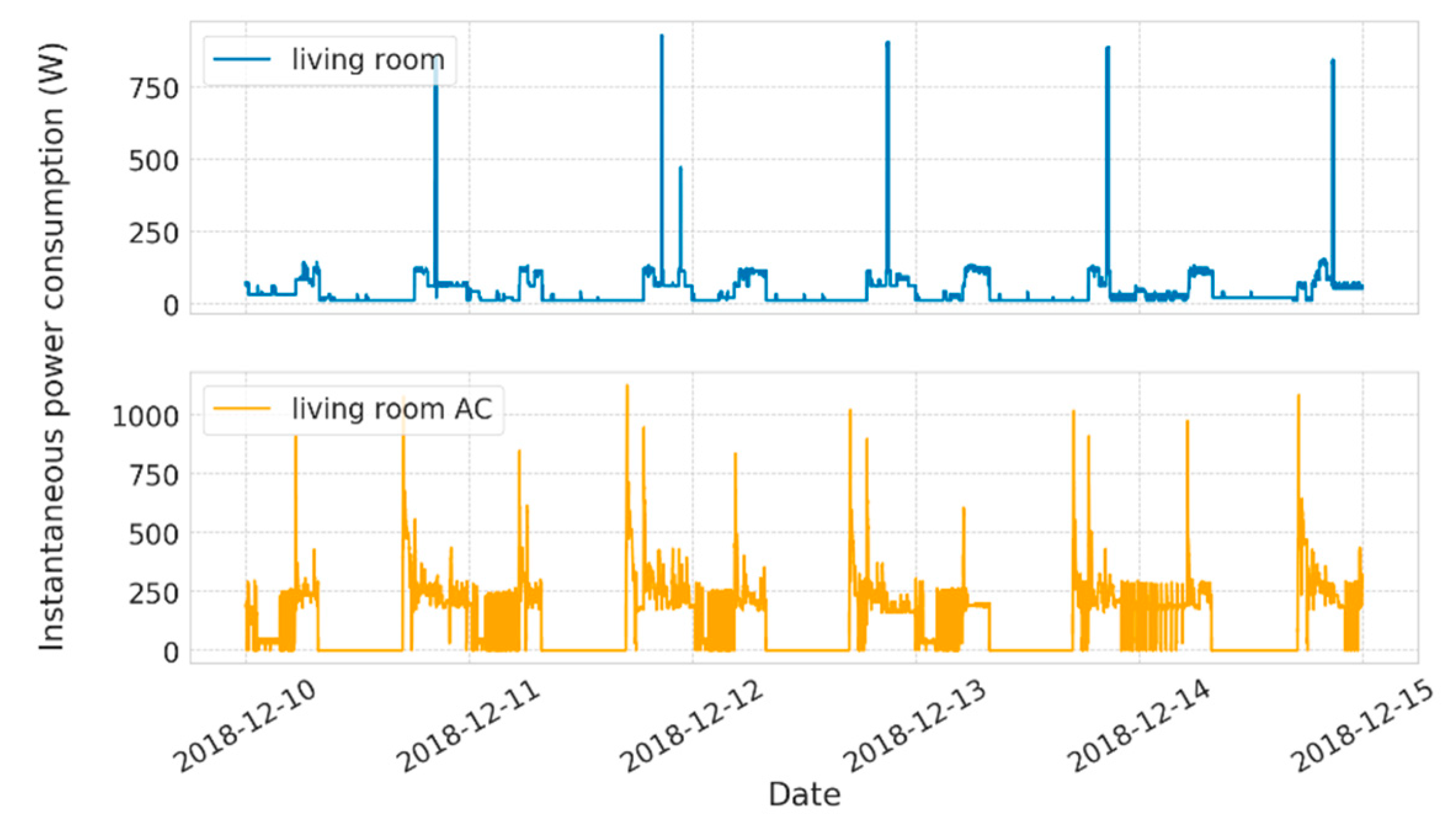
In a previous study [25], other inputs such as electricity consumption of home appliances are also discussed. Monitoring electricity usage in the real environment, we observed electricity consumption for electric appliances in the living room around 60 Wh on average. Figure 1 illustrates power consumption measured for electric plugs in the living room (top) and the AC (bottom).
The data is measured for each branch of the distribution board by an energy measuring unit. Comparing to other heat sources, the power consumption of electric appliances is relatively small. In addition, we observed that this value is similar to other houses. When houses with similar lifestyles are compared, it tends to be close between different houses. The similar degree of error in Ua estimation is considered when the power consumption of electric appliances is ignored. We assume the application of housing assessments for retrofit schemes. Since the same degree of assumed error is involved, the impact of this error is considered to be small when estimated Ua is compared between different houses. Therefore, we consider that the heat supply by electricity consumption of these appliances is relatively small compared to other inputs and can be ignored in the model. Here, we consider the total heat supply to the living room, , as in Equation (5).
2.1.6. Proposed Grey-Box Models
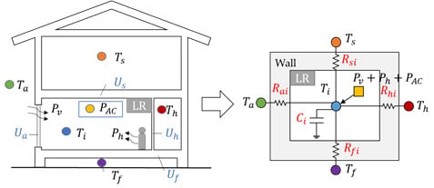
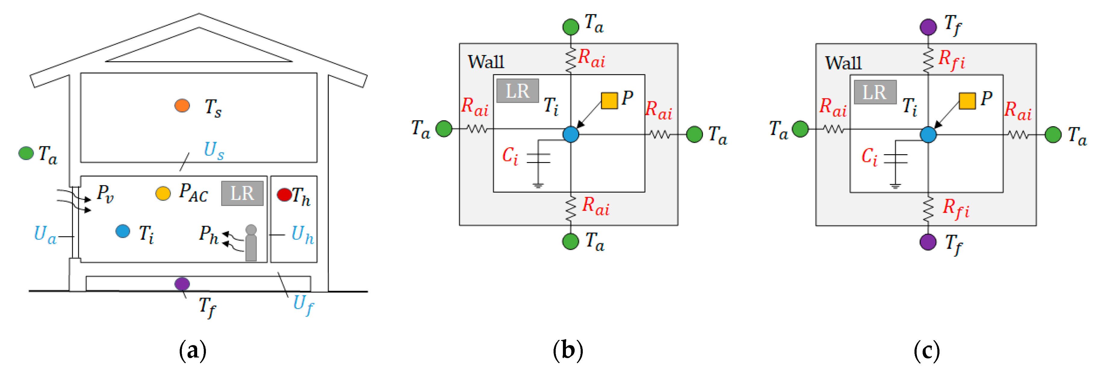
The grey-box models representing heat exchange for the living room are given in Equations (6)–(9). We propose four different models, namely, one-, two-, three-, and four-room models by detailing the model. They are expressed as analogies to RC circuit networks. The thermal resistance, is identical to electric resistance. Heat capacity is identical to electric capacitance. Figure 2a illustrates the inputs for heat exchanges of a house, while Figure 2b,c show the corresponding RC circuit network representation of the one- and two-room models. Other proposed models of three-, and four-room models can be represented in the same manner.
One-room model: This is the simplest 1R1C model and is given the inputs of , as shown in Equation (6):
where is the heat capacity of the living room. The temperatures outside the walls adjacent to the second floor, underfloor, and the hallway are represented by (Figure 2b).
Two-room model: This 2R1C model is given the inputs of as shown in Equation (7).
The temperature outside the wall adjacent to the second floor is represented by . The temperature outside the wall adjacent to the hallway is represented by (Figure 2c).
Three-room model: This 3R1C model is given the inputs of as shown in Equation (8).
The temperature outside the wall adjacent to the hallway is represented by (Figure 2c).
Four-room model: This 4R1C model is given the inputs of as shown in Equation (9).
2.2. Parameter Estimation
Estimating the unknown parameters in Equations (6)–(9) (i.e., heat capacity, and thermal resistances, ), is equivalent to solving system identification problems. In published studies, the methods of parameter estimation for house thermal model parameters typically use maximum likelihood estimations [23,24,26,31,32], the Bayesian approach [33,34], least squares minimization [25], and Kalman filter [35].
For establishing a low-cost method, reducing the computational effort to estimate unknown parameters is favorable. Thus, maximum likelihood estimations and Bayesian approaches are not appropriate. In addition, the parameter estimation method should cancel the effect of noise in the measured data since application in real environment is considered. The noise may include measurement errors of sensors. Therefore, a Kalman filter is used to estimate the parameters based on a published theory [36]. Here, we use the example of one-room model. Note that the same procedure is used for other models. Equation (6) is transformed for the equation of predicting room temperature of the living room, , by periods to give an equation as stated in Equation (10).
Then, the state and observation equations can be expressed as in Equations (11) and (12), respectively:
where , is process noise, and R is observation noise.
The observation of the system is , the Kalman filter estimates unknown parameters successively to minimize the difference between the predicted and measured . Note that the estimation method can also be applied to multiple room models in the same manner.
2.3. Model Validation
The proposed model is evaluated by using both estimation accuracy in Ua values and prediction errors in . In this section, the method of assessing prediction errors in is explained. The prediction error at time , , is defined as Equation (13), where is the predicted at , using estimated parameters of and .
Then, the assessment index, the average residual, , is introduced. This is calculated as the root mean square error (RMSE) of as represented in Equation (14):
where is the total number of data samples.
2.4. Data Selection and Pre-Processing
Unknown parameters are estimated for a continuous period of time when the AC is working. There are some uncertainties in the estimated parameters, owing to noise in the data. The dominant sources of the disturbances are occupant behaviors and AC characteristics. To avoid these disturbances, several approaches are proposed.
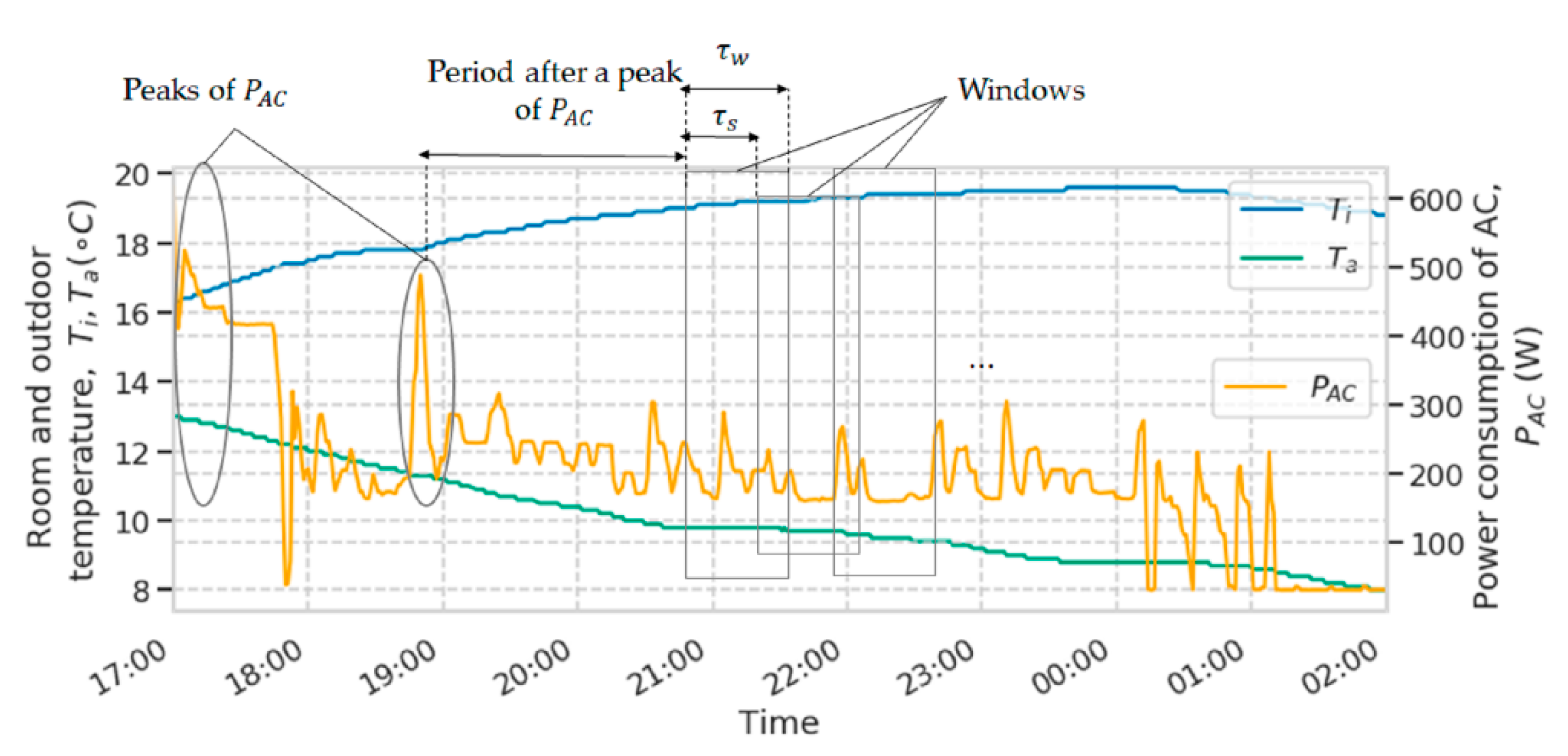
The disturbance caused by occupant behaviors can be decomposed into the change in the number of occupants and open windows. When these behaviors impact the thermal condition of the building, sudden changes in the room temperatures occur. We observed that when the room temperature changes suddenly, the AC changes its power input to control temperatures. From Figure 3, two peaks in can be observed around 17:00 and 19:00. After these peaks, we also observe fluctuations in and a steeper increase in . We consider that changes in the room environment may induce a change in the AC operation. It is also known that the variation in the COP of ACs depends on the power consumption. Right after the AC starts functioning, more variation in is observed. We observed that the indoor temperature tends to stabilize after the AC works for more than 2 h. Therefore, data right after the AC starts functioning are avoided to eliminate disturbances caused by both the occupant behavior and variation in the COP of ACs. In this study, periods where the AC functions for more than 2 h after observed peaks are chosen.
Finally, data windows of size are periodically generated at the interval of (practically, ). Figure 3 briefly describes the data preprocessing method. After 2 h from the second peak of for estimating under the stable AC operation, data windows are created (at ). The first data window is created for data between and . Then the second data window is created for data between and .
Unknown parameters are estimated for each window. Therefore, the final estimation values are presented as a distribution of estimated values per each data window. This method can reduce the impact of unexpected noise in short periods to the overall results. In addition, by using data windows, continuous usage of ACs for long periods is not required. In realistic situations, ACs are likely to get turned on and off several times a day. Our method does not require occupants to adjust their behaviors for the assessments.
Increasing means increasing the number of data windows created that may reduce the impact of noises. At the same time, reducing is important in the perspective of reducing computational effort. impacts the estimation performance of Kalman filter. Shorter the , Kalman filter may not converge to estimate the accurate parameter. Although longer is favorable, since the continuous operation time of the AC may be limited, shorter can create more data windows for calculation.
3. Experimental Design
3.1. Simulation Data
Simulation data is generated by a simulation tool, BEST (building energy simulation tool) [37]. BEST can simulate building thermal environments and energy consumption by allowing changes in parameters of the building envelope design and schedules of operation of HVAC appliances and occupant number.
The simulation is designed for a two-story, wooden detached house with a total floor area of 106 m2, with a living room area of 46 m2. The simulation assumes a uniform temperature in each room (i.e., living room, second floor, and underfloor). Three different envelope types are designed according to three different criteria, energy efficiency building standards in Japan for 1992 (denoted as H4), 1999 (H11), and HEAT20 G2 standards (HEAT20 G2), as given in Table 2. The transmission heat transfer coefficients for inner walls are designed as 2.18 W/m2K for all the simulation settings.
Twenty-four-hour ventilation systems with a constant ventilation rate of 64 m3/h and the AC with a COP of 3.6 are equipped in the living room. Note that the AC is operated for 24 h. The simulation considers two occupants with clothing with a clo value of 1. The Extended AMeDas Weather Data of Tokyo, Japan in 2010 [38] is used as the weather data. The simulation gives the output data with resolution of 5 min.
3.2. Experimental Data
The configuration of the data acquisition system should be simple and low-cost to achieve the requirements. Most data should be retrieved from the ACs and other low-cost sensors such as thermometers. However, we installed rich IoT sensors to evaluate our proposed method.
We used data from four different houses designed for the same criteria of energy performance. Data were collected from houses in a smart town in the Misono district, Saitama City, Japan. The smart town project, Urban Design Center Misono (UDCMi), was launched in 2016 in this district. The area of the district is 320 ha, and the planned population is 31,000. Several smart city services are proposed and adopted. In residential areas, home energy management systems (HEMS) are installed in smart houses to aggregate several kinds of data.
3.2.1. Experimental Settings
Figure 4 briefly explains the implemented HEMS. Sensor data are aggregated by a home gateway implemented on a Raspberry Pi 2 Model B via XBee. Then, the gateway sends the data to an IEEE1888 server over a virtual private network (VPN) tunnel. Rich kinds of environmental sensors are installed to measure data such as temperature, humidity, luminosity, dust, and CO2. A BLE beacon is placed in the living room. Data of AC power consumption are collected via energy measuring units, HEM-EME5A. These are attached to the distribution boards of houses to measure the electric consumption of each electric branch. A program written in JavaScript is used to retrieve electric branch data via ECHONET Lite Version1.10. The resolution of environmental and electrical data is 1 min.
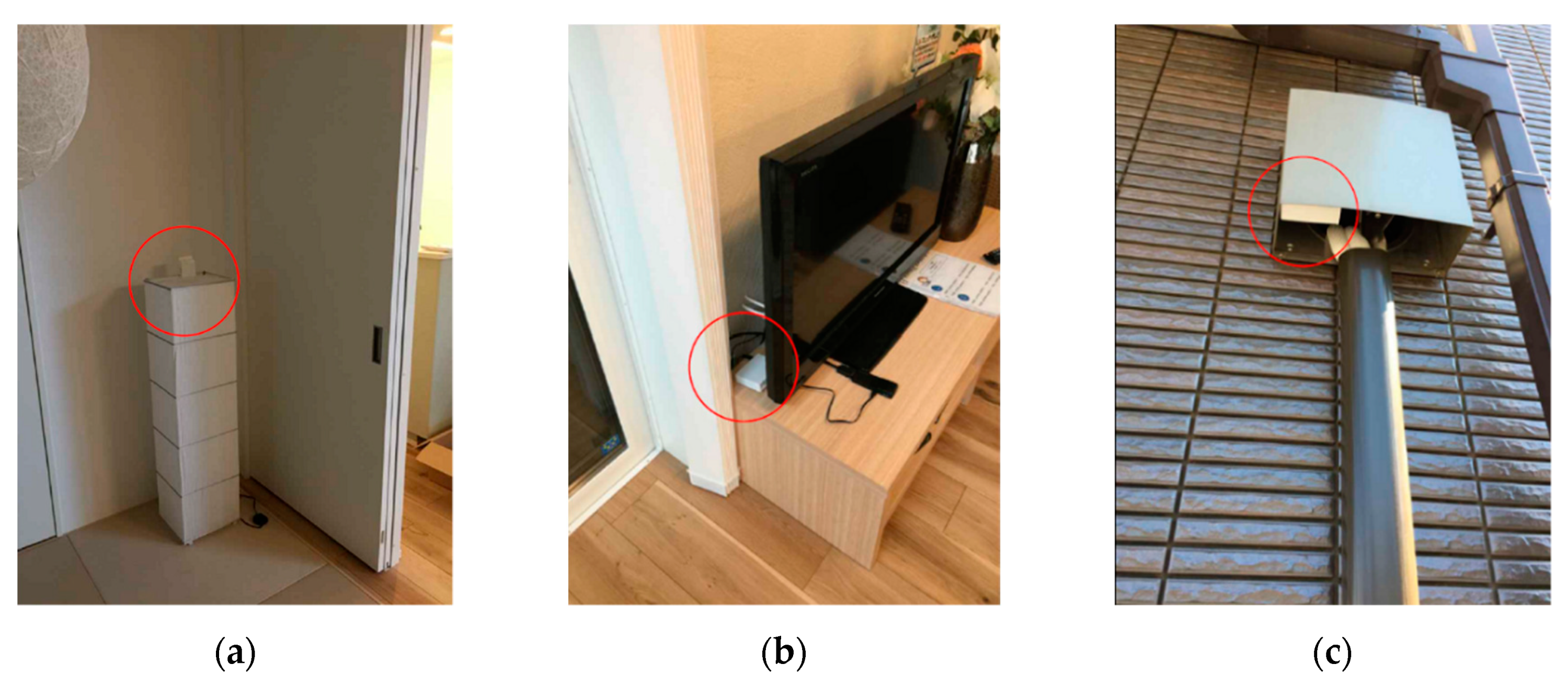
Figure 5 shows examples of the installment of different environmental sensors for UDCMi. Environmental sensors should be equipped to achieve accurate measurement. However, at the same time, the installment location should be chosen to not disturb residents. Thermometers are located 800–1300 mm above the floor, away from windows and outer walls (Figure 5a). They also are placed to avoid direct heat from the ACs to measure values close to average room temperatures. CO2 and dust sensors are installed away from windows (Figure 5b). Thermometers to measure outdoor temperature are placed on gutters, 2000–2500 mm above the ground (Figure 5c), avoiding direct solar radiation and rains (north sides are preferred). They are also away from the outdoor units of the ACs. We selected air temperature instead of globe temperature or static air temperature (SAR), which the ACs can measure. Air mixing is also abbreviated. It is true that the effects of solar radiation, nocturnal radiation, and heat storage are not ignorable on the temperature measurement. However, we assume these effects are small for data retrieved during nighttime.
3.2.2. Household Information
Four target houses (Home 1 to 4) were constructed during the same period under the strict criteria of the house thermal performance HEAT20 G2 with Ua values of 0.45 W/m2K. These houses have a similar building plan. A large part of the ground floor consists of a living room. The total floor area ranges 90–110 m2. The occupant number is 2 adults (Home 4) or two adults and one child (Home 1, 2, and 3). All data were collected from 10–31 December 2018. Home 1 to 4 are equipped with the ACs. The COP values are assumed to be 3 as it is typical value for the ACs installed in the living rooms.
4. Results and Discussion
Our proposed method was thoroughly assessed using both simulation and experimental data. Simulation data were used to evaluate if our proposed method satisfied the stated requirements for housing assessments. Experimental data retrieved from real settings of houses occupied by residents were used to further assess if our proposed method can be applied in real settings.
All evaluation results were derived by setting the parameters for the window size, , as 2 h and the window interval, , as 30 min. A preliminary experiment was performed to confirm that setting smaller than 60 min gives similar results. Evaluation on is presented in Section 4.2.1. The observation noise is set as 0.1 from the measurement error of thermometers. The process noise, where corresponds to the noise for is determined from the variation in observed value of .
4.1. Thermal Performance Estimation using Simulation Data
Ua value estimation using two-, three-, and four-room models was conducted using fixed values for the thermal resistances to the adjacent rooms (i.e., ) as represented in Table 2. This is because an intensive adjustment in initial values of parameters is required when all the thermal resistances are identified for multi-room models. This identification difficulty is caused by small differences in temperature between the living rooms and their adjacent rooms. As we can still achieve the purpose of accurate estimation of Ua values, we identified Ua values using fixed values for the thermal resistances to the adjacent rooms.
4.1.1. Evaluation of Estimated Thermal Performance
The thermal performance of building envelopes is estimated using 10 days (between January 1 and January 10) of the three different simulation data (i.e., HEAT20 G2, H11, and H4 standards). These data include the coldest day of the year, with stable weather conditions.
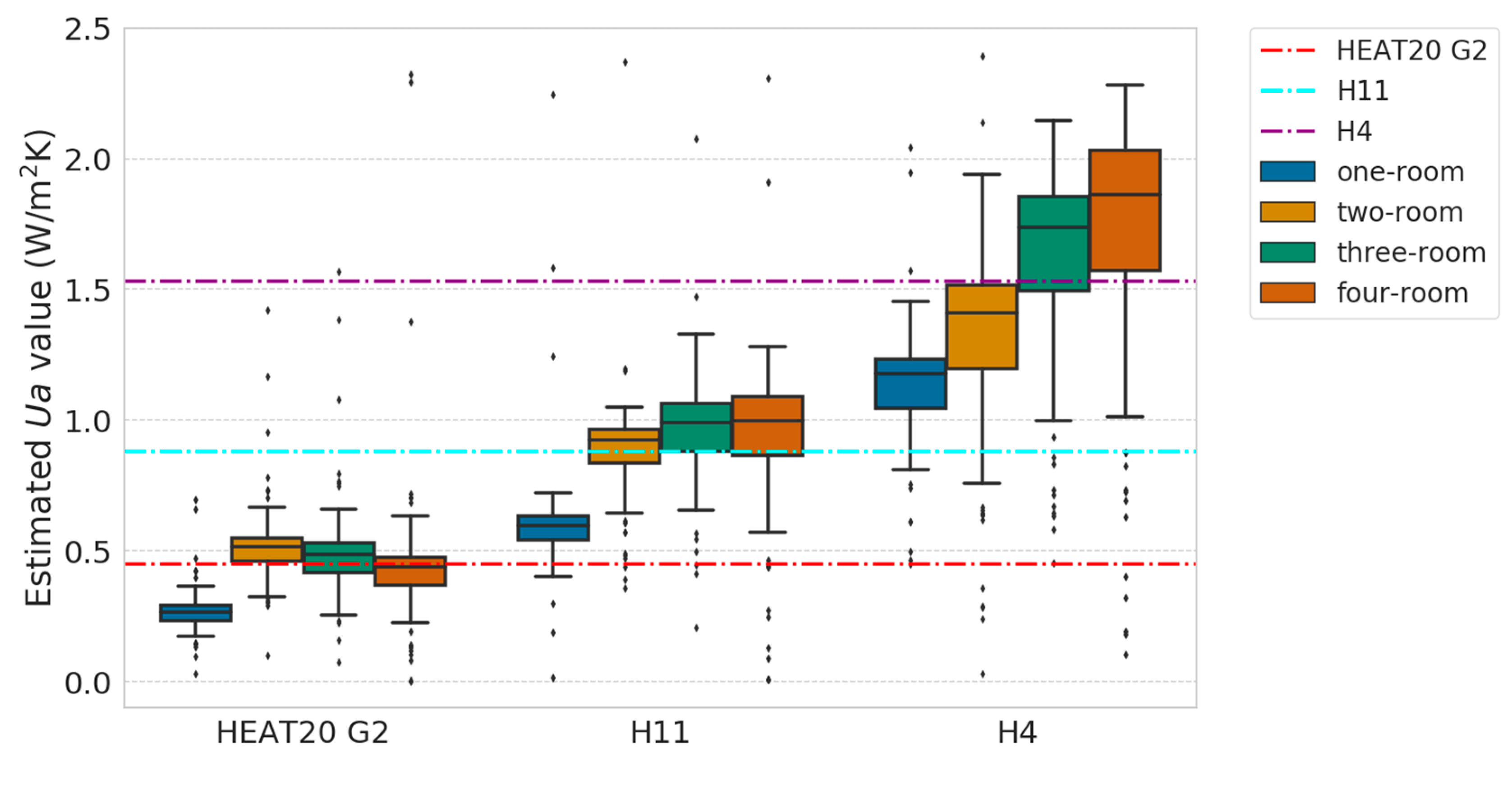
Hundred-twenty-six data windows are obtained for the estimation of Ua values. The identified parameters are obtained as the distribution of estimated values for each corresponding data window as presented in Figure 7. The estimated Ua values are compared to the literature values which are calculated from the physical properties of construction materials.
The estimation results for two-, three-, and four-room models show good accuracy compared to the literature Ua values for each simulation data. The results for HEAT20 G2 show the best accuracy for all data. However, the results for H4 show more difference between literature and estimated values than the other data, especially for the four-room model. By detailing the model, Ua values are overestimated from the literature values because of the high transmission heat transfer coefficient of windows, especially for the H4 standards. The living room windows are relatively large. By considering adjacent rooms to floors and ceilings for the detailed model, the gap of thermal performance between the window and outer walls has a greater impact on the estimated Ua values. Since the designed transmission heat transfer coefficients are larger for the windows in low thermal performance houses, their Ua values are likely to be overestimated. The summary of the median of estimated thermal performance parameters for each simulation data is presented in Table 3.
Average residuals for each simulation data and model are presented in Table 4. For all models and data, the average residuals are relatively small, achieving order while the measuring order is . This indicates good performance in parameter identification and in predicting the of the proposed models. The average residual is slightly larger for the one-room model than other models for H11 and H4 standard. This may be because of the greater impacts of outdoor temperature dynamics to the temperature of the living room and its adjacent rooms. However, the difference in the average residual for each model is very small. Therefore, two- and three-room model are considered to be suitable because they show good performance in estimating Ua values that are close to the literature value.
Comparing different simulation data, average residuals for HEAT20 G2 are the smallest, followed by H11 and H4, showing better performance of the proposed methods for houses with higher thermal performance. This is considered due to more variation in input data for houses with lower thermal performance. This variation, i.e., more noise in the data, may lower the estimation accuracy. In the same manner, the results for H4 data show larger variation in estimated Ua values, as shown in Figure 7. The major factor that induces the estimation errors is considered as the characteristics of the AC power inputs. Under certain conditions, we observed that the AC power inputs fluctuate. The analysis of errors is conducted in the next section from the perspective of selecting appropriate data to achieve estimation accuracy.
4.1.2. Analysis of Estimation Errors for Simulation Data
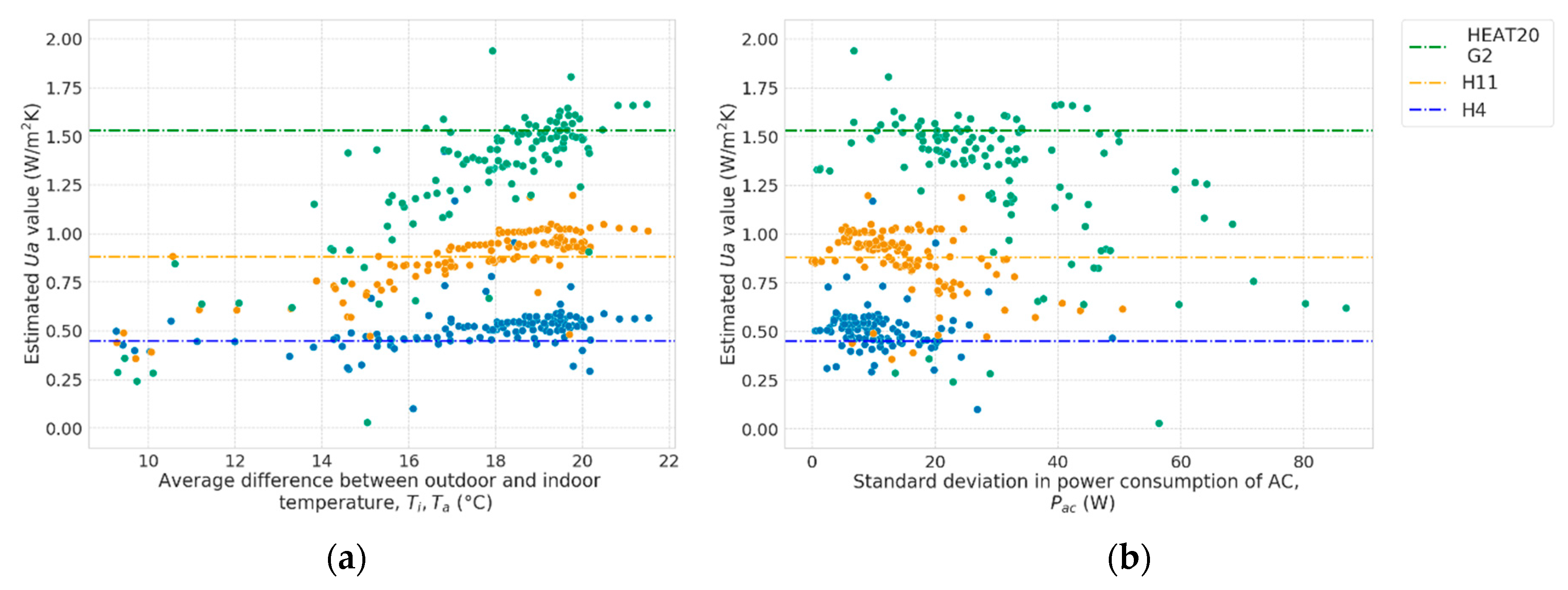
Analysis in the previous section gave insights into how some conditions may lead to estimation errors, which is in agreement with previous studies [33,39,40]. We have investigated the impacts of temperature difference on the estimation performance of our proposed methods using different simulation data. The analysis results for the two-room model are shown for brevity, but the results for other models show similar trends. The scatter plot in Figure 8a represents the correlation between estimated Ua values (y-axis) and the average difference between indoor and outdoor temperature (, respectively) for different standards. Results for H4 indicate that estimated Ua values decrease as the average difference in outdoor and indoor temperature decreases. Larger errors are observed when the difference between outdoor and indoor temperature is smaller. This trend is less noticeable for houses with better thermal performance, such as HEAT20 G2.
The characteristics of AC operation in houses with different thermal performance further explain the errors. We observed fluctuation in power consumption of the ACs within data windows that may induce the estimation errors. Figure 8b shows the relationship between estimated Ua values (y-axis) and the standard deviation in power consumption of the AC () (x-axis) for different simulation data. When the standard deviation of increases, there is more variation in estimated Ua values. This trend is more apparent for H4 than for other data. In addition, standard deviations of for H4 are larger overall than other data, which means more variation in power inputs into the living room. Therefore, fluctuation in AC power input can result in estimation errors for Ua values.
There is a correspondence relationship between estimated Ua values and the temperature difference between outdoor and indoor temperature. We observe that when the temperature difference between indoor and outdoor temperature is smaller (i.e., when the indoor environment is not heated enough), the AC is likely to increase power consumption to heat the rooms. The dynamic range of room temperature is more drastic at the beginning of AC operation before more constant conditions are achieved, which explains the larger errors for H4 because larger thermal dynamics are induced by lower thermal performance. Therefore, the data having both larger differences between outdoor and indoor temperature and stable AC power input should be used for thermal performance estimations.
4.1.3. Thermal Performance Estimation Before and After Retrofits
Further evaluation of our proposed method is performed on the estimation of building thermal performance before and after retrofits. Three different cases of partial retrofits are simulated: That of insulating outer walls, that of replacing windows in the whole house, and that of replacing windows only in the living rooms. For brevity, the simulation results of the house designed under the criteria of H11, discussed in Section 3.1, are presented. The detailed thermal performance of walls is given in Table 2. Insulating materials commonly used for walls are phenolic forms [41], which improve the transmission heat transfer coefficient of outer walls from 0.53 to 0.41 W/m2K. The windows are replaced to energy-efficient double-glazed glass [42], improving the performance from 4.65 to 2.33 W/m2K. The results for three-room model are shown in Table 5.
The estimated results show the performance of our proposed method when building materials are partially replaced. The relative error for estimation results before retrofits is 9.1%. The estimation performance is better for when larger areas of materials are replaced for a house, as the relative errors to the literature values are 3.6% and 6.1% when retrofitting outer walls and all windows, respectively. When replacing only the living room’s windows, the relative error increases to 16.7%. This may be caused by the large percentage of windows that are placed in the living rooms. The thermal performance of the windows in the living rooms is critical to the thermal performance of the whole house. However, the results indicate that our estimation methods can provide information on the degree of improvements in thermal performance to residents after retrofits.
4.2. Thermal Performance Estimation using Experimental Data
4.2.1. Evaluation of Thermal Performance Estimation
Data retrieved during nighttime hours (18:00–05:00) were used for thermal performance estimation with experimental data. Estimation was conducted considering only 24 h ventilation systems and one occupant in the living room for all houses. The COP values of the ACs were considered constant. Note that although variability in ventilation rate and the number of occupants within a house are not ignorable, we use fixed values for these uncertainties. Since our proposed method aims for simple in situ measurements using a reduced number of sensors, we assess the thermal performance of the houses while allowing some uncertainties in data. This is reasonable because we can compare the thermal performance of different houses by considering the fixed values of these uncertainties. This strategy is useful for selecting houses to join retrofit schemes. In addition, the output of thermal performance estimation for housing assessments should include the performance gap from designed values that is induced by these uncertainties.
Figure 9 presents the estimated parameters derived by different models for four houses. For all the houses, the median of estimated Ua values of two- and three-room models exhibit good correspondence to literature Ua value of 0.45 W/m2K (a literature value for heat capacity, , is not given), which suggests the performance of our proposed method in estimating Ua values also applies to experimental data. The four-room model shows different trends relative to the other models. The estimated Ua values are smaller than two- and three-room models for Home 3 and 4, similar to the simulation results, but larger for Home 1 and 2. This may be caused by different usage of rooms for each house. The four-room model considers adjacent rooms of the hallway on the first floor, but the three-room model only considers the second floor and the underfloor. In real-life settings, air exchange between the living room and the hallway is more likely to occur than between the living room and the second floor or the underfloor. In the four-room models, air exchange between different rooms is not considered. This discrepancy between assumptions and actual situations causes the low performance of the four-room models.
Table 6 and Table 7 summarize the median of estimated parameters ( and ) and average residuals (), respectively. The average residuals are calculated as 10−2 to 10−1 order. As the measurement error of the thermometers is 0.1, this is considered relatively small. Similarly to the simulation results, the average residuals for each model exhibit similar values. Since the estimated Ua values for two- and three-room models were close to the literature value, good estimation performance of these models is shown for experimental data as well. Table 8 summarizes the information on AC operation for each house. Longer average operation time for the AC is observed for Home 2 than for other houses. We select data which AC operates for more than 2 h. This infers that more data samples are available for houses with longer AC operation that may increase the overall accuracy in Ua estimation. The tradeoff in selecting appropriate window size is considered here. While using larger window size can increase parameter estimation performance, the number of data windows decreases.
The estimation is performed for different size of data window, . Figure 10 presents the estimated Ua value for different size of the data window. Only the results for Home 4 using three-room model is presented for brevity but other cases exhibit similar results. The interval of data window, is set as 30 min. We can observe that larger the value of , smaller the variation in the estimated Ua values. Results with larger than 2 h present smaller interquartile range. Considering the average operation time of the ACs, which is around 3–5 h, setting around 2–3 h is reasonable. This also exhibits the feasibility of our proposed method to accurately estimate Ua values using real AC operation data.
4.2.2. Analysis of estimation errors for experimental data
Estimation errors are considered to be induced by the variation in input power of ACs, ventilation rate, and the number of occupants. In this section, we focus on the impacts of characteristics in AC operations when the number of occupants changes. Although the impacts of ventilation are not ignorable, we did not observe major errors that seem to be induced by ventilation. We consider that since data were collected during winter nighttime, ventilation activity such as opening windows was not likely to occur.
Analysis of estimation errors was conducted using data retrieved from Home 4. Only the results for the two-room model are presented in this section for brevity. We observed similar trends for all other models. Figure 11a presents the relationship between estimated Ua values (y-axis) and the standard deviation in power consumption of the AC, (x-axis). When the standard deviation of is above its upper quartile (66 W), larger Ua values are observed. This confirms the observation from the previous section that increases in the fluctuation of induces estimation errors. However, the trend is opposite from the simulation results, while larger fluctuations in corresponded to lower estimated Ua values in simulations, larger Ua values were obtained with experimental data. One reason for this discrepancy with the simulation results is the effect of variation in COP values. The efficiency of AC operations is known to vary depending on their power consumption. AC operations achieve better efficiency with higher power consumption. Since we use data for 2 h after initiation of the AC, we observe fluctuations in AC power when the room is overheated and the AC decreases its input. Figure 11b explains this behavior of the ACs in real settings. When the average (y-axis) decreases, the standard deviation of (x-axis) increases. This corresponds to the characteristic of COP that when the power consumption is low, the efficiency in the AC decreases, inducing overestimation of the Ua values.
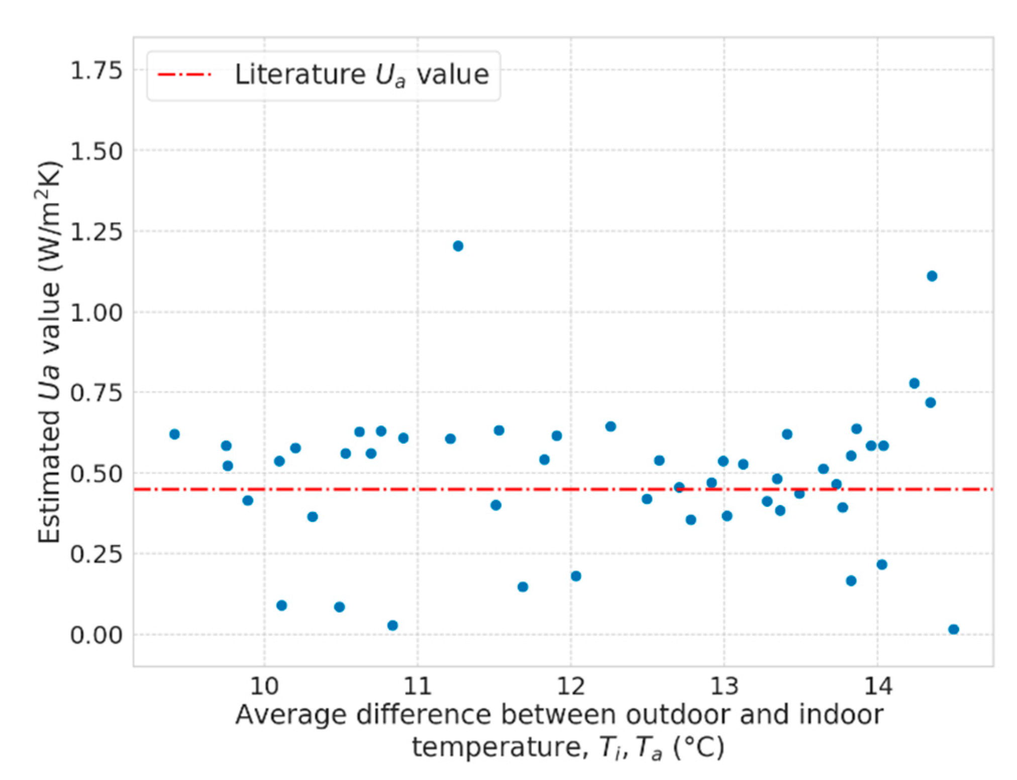
Figure 12 represents the relationship between estimated Ua values (y-axis) and the average difference between outdoor and indoor temperature (x-axis) for data with a standard deviation of PAC that is smaller than its upper quartile. When the average difference between outdoor and indoor temperature is smaller, larger Ua values are obtained. Note that this result is not induced by fluctuations in PAC since data with the larger standard deviation of PAC are removed. One of the error sources may be the variation of COP values. It is known that the COP value of ACs variate depending on their power consumption. When the power consumption is small, the efficiency may be low. COP value at the best efficiency is used as the catalog value. Although actual COP values variate, they are treated as constant. This explains the observation. When the difference in outdoor and indoor temperature is small, the power consumption of the AC may be smaller that lowers the efficiency and the Ua value is estimated larger.
5. Conclusions
This paper proposed thermal performance estimation methods for detached houses using ACs. Thermal dynamics of houses are mathematically modeled using grey-box models. Data selection and preprocessing techniques are then proposed to achieve thermal performance assessment under limited conditions in real settings. Proposed methods are evaluated thoroughly using both simulation and experimental data. Our proposed method satisfies the requirements for housing assessments for retrofits as follows:
- Accurate: Simulation results show estimation accuracy of the proposed method for houses with different thermal performance. The proposed two- and three-room models exhibit good estimation accuracy for all data. For example, accuracy with 13.7% relative error was obtained for the house with a Ua value of 1.35 Wm2K as the worst case. The assessment results using experimental data also showed good correspondence to the literature Ua values. Further, an analysis in errors was conducted and indicated that the characteristics of AC operation may induce estimation errors. The error analysis inferred that the major factor that induces the estimation error is variation in COP. Although detailed information on COP variation is often not revealed by the manufactures, further analysis of COP variation of the ACs may give insights to its impacts on estimation errors.
- Low installment cost: The system can be implemented in low-cost. For example, to estimate Ua values using the three-room model, we only require information on the electricity consumption of the ACs, temperatures of the living room, second floor, and outdoors, and occupancy. The total cost for the system would be below $150 that achieves the requirements.
- Simple and undemanding to residents: As mentioned, the system only requires an AC, a gateway, communication modules, and an additional thermometer. The system is simple and does not disturb the residents. Once the sensors are placed, assessments are done remotely without assistance from the residents.
By satisfying the requirements, our proposed method can be used as a tool to select houses which benefit from joining retrofit schemes in a cost-effective way. The thorough evaluation demonstrated the capability of our proposed method to estimate Ua values for detached houses. Our proposed method may be expanded for other archetypes in the future. Since only one additional sensor is required other than an AC, our proposed method may be applied as an inherent function of AC units that can continuously monitor building thermal performance even after the retrofits.
Author Contributions
Conceptualization, Y.S. and H.N.; methodology, Y.S. and H.N.; software, Y.S.; validation, Y.S. and H.N.; formal analysis, Y.S.; investigation, Y.S.; resources, H.N.; data curation, Y.S. and H.N.; writing—original draft preparation, Y.S.; writing—review and editing, H.N.; visualization, Y.S.; supervision, H.N.; project administration, H.N.
Acknowledgments
This work was supported by MEXT/JSPS KAKENHI Grant B) Number JP16H04455 and JP17H01739.
Conflicts of Interest
The authors declare no conflict of interest. Additionally, the funders had no role in the design of the study; in the collection, analyses, or interpretation of data; in the writing of the manuscript; or in the decision to publish the results.
References
- Iwafune, Y.; Yagita, Y. High-resolution determinant analysis of Japanese residential electricity consumption using home energy management system data. Energy Build. 2016, 116, 274–284. [Google Scholar] [CrossRef]
- National Diet Library, Issue Brief—Green New Deal in Foreign Countries: Creation of Industry and Employment by Environment. Available online: http://www.ndl.go.jp/jp/diet/publication/issue/0641.pdf (accessed on 7 July 2019).
- Sustainable Open Innovation Initiative. Available online: http://sii.or.jp/ (accessed on 7 July 2019).
- Less, B.; Walker, I. A Meta-Analysis of Single-Family Deep Energy Retrofit Performance in the U.S.; Lawrence Berkeley National Laboratory: Berkeley, CA, USA, 2014. [Google Scholar]
- Kampelis, N.; Gobakis, K.; Vagias, V.; Kolokotsa, D.; Standardi, L.; Isidori, D.; Venezia, L. Evaluation of the performance gap in industrial, residential & tertiary near-Zero energy buildings. Energy Build. 2017, 148, 58–73. [Google Scholar] [Green Version]
- Ficco, G.; Iannetta, F.; Ianniello, E.; Romana D’, F.; Alfano, A.; Dell’isola, M. U-value in situ measurement for energy diagnosis of existing buildings. Energy Build. 2015, 104, 108–121. [Google Scholar] [CrossRef]
- Marshall, A.; Fitton, R.; Swan, W.; Farmer, D.; Johnston, D.; Benjaber, M.; Ji, Y. Domestic building fabric performance: Closing the gap between the in situ measured and modelled performance. Energy Build. 2017, 150, 307–317. [Google Scholar] [CrossRef]
- Ferrarini, G.; Bison, P.; Bortolin, A.; Cadelano, G. Thermal response measurement of building insulating materials by infrared thermography. Energy Build. 2016, 133, 559–564. [Google Scholar] [CrossRef]
- Lee, S.; Kato, S. Feasibility study of in situ measurement method using the infrared camera to measure U value of walls on residential house installed an convection stove. Jpn. Environ. Eng. AIJ 2011, 76, 289–295. [Google Scholar] [CrossRef]
- Tejedor, B.; Casals, M.; Gangolells, M.; Roca, X. Quantitative internal infrared thermography for determining in-situ thermal behaviour of façades. Energy Build. 2017, 151, 187–197. [Google Scholar] [CrossRef]
- Tejedor, B.; Casals, M.; Gangolells, M. Assessing the influence of operating conditions and thermophysical properties on the accuracy of in-situ measured U-values using quantitative internal infrared thermography. Energy Build. 2018, 171, 64–75. [Google Scholar] [CrossRef]
- Atsonios, I.A.; Mandilaras, I.D.; Kontogeorgos, D.A.; Founti, M.A. A comparative assessment of the standardized methods for the in–situ measurement of the thermal resistance of building walls. Energy Build. 2017, 154, 198–206. [Google Scholar] [CrossRef]
- Bauwens, G.; Roels, S. Co-heating test: A state-of-the-art. Energy Build. 2014, 82, 163–172. [Google Scholar] [CrossRef]
- Cesaratto, P.G.; De Carli, M. A measuring campaign of thermal conductance in situ and possible impacts on net energy demand in buildings. Energy Build. 2013, 59, 29–36. [Google Scholar] [CrossRef]
- Johnston, D.; Miles-Shenton, D.; Farmer, D. Quantifying the domestic building fabric ‘performance gap’. Build. Serv. Eng. Res. Technol. 2015, 36, 614–627. [Google Scholar] [CrossRef]
- Giraldo-Soto, C.; Erkoreka, A.; Mora, L.; Uriarte, I.; del Portillo, L.A. Monitoring system analysis for evaluating a building’s envelope energy performance through estimation of its heat loss coefficient. Sensors 2018, 18, 2360. [Google Scholar] [CrossRef] [PubMed]
- Márquez, J.M.A.; Bohórquez, M.Á.M.; Melgar, S.G.; Andújar Márquez, J.M.; Martínez Bohórquez, M.Á.; Gómez Melgar, S. A New Metre for Cheap, Quick, Reliable and Simple Thermal Transmittance (U-Value) Measurements in Buildings. Sensors 2017, 17, 2017. [Google Scholar] [CrossRef] [PubMed]
- Farmer, D.; Gorse, C.; Swan, W.; Fitton, R.; Brooke-Peat, M.; Miles-Shenton, D.; Johnston, D. Measuring thermal performance in steady-state conditions at each stage of a full fabric retrofit to a solid wall dwelling. Energy Build. 2017, 156, 404–414. [Google Scholar] [CrossRef]
- Alzetto, F.; Pandraud, G.; Fitton, R.; Heusler, I.; Sinnesbichler, H. QUB: A fast dynamic method for in-situ measurement of the whole building heat loss. Energy Build. 2018, 174, 124–133. [Google Scholar] [CrossRef]
- Thébault, S.; Bouchié, R. Refinement of the ISABELE method regarding uncertainty quantification and thermal dynamics modelling. Energy Build. 2018, 178, 182–205. [Google Scholar] [CrossRef]
- Yanagisawa, Y.; Inayama, M.; Mae, M.; Aoki, K.; Sawai, H. Study on presumption of heat loss factor by simple field measurement of wooden houses. AIJ J. Technol. Design 2016, 22, 591–596. [Google Scholar] [CrossRef]
- Bacher, P.; Madsen, H. Identifying suitable models for the heat dynamics of buildings. Energy Build. 2011, 43, 1511–1522. [Google Scholar] [CrossRef] [Green Version]
- Deconinck, A.H.; Roels, S. Is stochastic grey-box modelling suited for physical properties estimation of building components from on-site measurements? J. Build. Phys. 2017, 40, 444–471. [Google Scholar] [CrossRef]
- Jiménez, M.J.; Madsen, H.; Andersen, K.K. Identification of the main thermal characteristics of building components using MATLAB. Build. Environ. 2008, 43, 170–180. [Google Scholar] [CrossRef]
- Van Leeuwen, R.P.; De Wit, J.B.; Fink, J.; Smit, G.J.M. House thermal model parameter estimation method for Model Predictive Control applications. In Proceedings of the 2015 IEEE Eindhoven PowerTech, Eindhoven, The Netherlands, 29 June–2 July 2015; pp. 1–6. [Google Scholar]
- Andersen, P.D.; Jiménez, M.J.; Madsen, H.; Rode, C. Characterization of heat dynamics of an arctic low-energy house with floor heating. Build. Simul. 2014, 7, 595–614. [Google Scholar] [CrossRef]
- Kim, D.; Cai, J.; Ariyur, K.B.; Braun, J.E. System identification for building thermal systems under the presence of unmeasured disturbances in closed loop operation: Lumped disturbance modeling approach. Build. Environ. 2016, 107, 169–180. [Google Scholar] [CrossRef] [Green Version]
- ECHONET. Available online: https://echonet.jp/english/ (accessed on 7 July 2019).
- Sakuma, Y.; Nakajo, Y.; Nishi, H. Building Thermal Performance Assessments Using Simple Sensors for the Green New Deal in Japan. In Proceedings of the IEEE International Symposium on Industrial Electronics, Cairns, QLD, Australia, 13–15 June 2018; pp. 691–696. [Google Scholar]
- Yan, Y.Y.; Oliver, J.E. The clo: A utilitarian unit to measure weather/climate comfort. Int. J. Climatol. A J. R. Meteorol. Soc. 1996, 16, 1045–1056. [Google Scholar] [CrossRef]
- Asdrubali, F.; Buratti, C.; Cotana, F.; Baldinelli, G.; Goretti, M.; Moretti, E.; Bevilacqua, D. Evaluation of Green Buildings’ Overall Performance through in Situ Monitoring and Simulations. Energies 2013, 6, 6525–6547. [Google Scholar] [CrossRef]
- Deconinck, A.H.; Roels, S. Comparison of characterisation methods determining the thermal resistance of building components from onsite measurements. Energy Build. 2016, 130, 309–320. [Google Scholar] [CrossRef] [Green Version]
- Gori, V.; Biddulph, P.; Elwell, C.; Gori, V.; Biddulph, P.; Elwell, C.A. A Bayesian Dynamic Method to Estimate the Thermophysical Properties of Building Elements in All Seasons, Orientations and with Reduced Error. Energies 2018, 11, 802. [Google Scholar] [CrossRef]
- Gori, V.; Elwell, C.A. Estimation of thermophysical properties from in-situ measurements in all seasons: Quantifying and reducing errors using dynamic grey-box methods. Energy Build. 2018, 167, 290–300. [Google Scholar] [CrossRef]
- Wang, X.; Wang, X. The comparison of particle filter and extended Kalman filter in predicting building envelope heat transfer coefficient. In Proceedings of the 2012 IEEE 2nd International Conference on Cloud Computing and Intelligence Systems, IEEE CCIS 2012, Hangzhou, China, 30 October–1 November 2012; Volume 3, pp. 1524–1528. [Google Scholar]
- Alspach, D.L. On the Identification of Variances and Adaptive Kalman Filtering. IEEE Trans. Auto. Control 1972, 17, 843–845. [Google Scholar] [CrossRef]
- The BEST PROGRAM Building Energy Simulation Tool—About BEST. Available online: http://www.ibec.or.jp/best/english/index.html (accessed on 7 July 2019).
- Meteorological Data System Co. Available online: https://www.metds.co.jp/ (accessed on 7 July 2019).
- Asdrubali, F.; D’Alessandro, F.; Baldinelli, G.; Bianchi, F. Evaluating in situ thermal transmittance of green buildings masonries—A case study. Case Stud. Constr. Mater. 2014, 1, 53–59. [Google Scholar] [CrossRef]
- Gaspar, K.; Casals, M.; Gangolells, M. In situ measurement of façades with a low U-value: Avoiding deviations. Energy Build. 2018, 170, 61–73. [Google Scholar] [CrossRef]
- Schiavoni, S.; D’alessandro, F.; Bianchi, F.; Asdrubali, F. Insulation materials for the building sector: A review and comparative analysis. Renew. Sustain. Energy Rev. 2016, 62, 988–1011. [Google Scholar] [CrossRef]
- Carbonara, E.; Tiberi, M. Assessing energy performance and economic costs of retrofitting interventions in a university building. In Proceedings of the EEEIC 2016—International Conference on Environment and Electrical Engineering, Florence, Italy, 7–10 June 2016; pp. 1–5. [Google Scholar]
Figure 1.
Power consumption of electric appliances in the living room (in blue) and the AC (in orange).
Figure 1.
Power consumption of electric appliances in the living room (in blue) and the AC (in orange).

Figure 2.
(a) Heat exchange for the living room (LR), (b) one-room model, (c) two-room model, where the measured inputs by sensors, ( are represented in circles, total heat supply to the living room () are in a square, unknown parameters of heat capacity () and thermal resistances () are in red texts, and heat transfer coefficients () derived from estimated parameters are in blue texts.

Figure 3.
Methods for data selection and preprocessing: The y-axis in the left and right represent temperature in the living room () and outdoor () and power consumption of the AC (), respectively, the x-axis represents time. Data windows with the size of are generated periodically ( after the previous window) 2 h after the peak of .

Figure 4.
House energy management system (HEMS) installed in smart houses for the Urban Design Center Misono (UDCMi) project. Environmental and electric data are collected at the gateway and sent to the server for storage. Various home services using these data are provided for UDCMi.
Figure 4.
House energy management system (HEMS) installed in smart houses for the Urban Design Center Misono (UDCMi) project. Environmental and electric data are collected at the gateway and sent to the server for storage. Various home services using these data are provided for UDCMi.

Figure 5.
Installment of environmental sensors: (a) A thermometer in the room, (b) CO2 sensor, (c) a thermometer on the outside north-facing wall. Sensors are circled in red.
Figure 5.
Installment of environmental sensors: (a) A thermometer in the room, (b) CO2 sensor, (c) a thermometer on the outside north-facing wall. Sensors are circled in red.

Figure 6.
Screenshots of the smartphone application: (a) Room environment information (b) electricity usage information.
Figure 6.
Screenshots of the smartphone application: (a) Room environment information (b) electricity usage information.

Figure 7.
Estimated Ua values for different simulation data (HEAT20 G2, H11, and H4) and models (one-, two-, three-, and four-room model). The dotted line represents literature Ua values for each standard. Boxplots represent the distribution of estimated results for the different models.
Figure 7.
Estimated Ua values for different simulation data (HEAT20 G2, H11, and H4) and models (one-, two-, three-, and four-room model). The dotted line represents literature Ua values for each standard. Boxplots represent the distribution of estimated results for the different models.

Figure 8.
Estimated Ua values and: (a) Average difference between outdoor and indoor temperature (), (b) standard deviation in power consumption of the ACs (). Dotted lines represent literature values for different standards (HEAT20 G2, H11, and H4).
Figure 8.
Estimated Ua values and: (a) Average difference between outdoor and indoor temperature (), (b) standard deviation in power consumption of the ACs (). Dotted lines represent literature values for different standards (HEAT20 G2, H11, and H4).

Figure 9.
Estimated Ua values for different experimental data (Home 1 to 4) and models (one-, two-, three- and four-room model). The dotted line represents the literature Ua value. Boxplots represent distribution of estimated results for the different models.
Figure 9.
Estimated Ua values for different experimental data (Home 1 to 4) and models (one-, two-, three- and four-room model). The dotted line represents the literature Ua value. Boxplots represent distribution of estimated results for the different models.

Figure 10.
Estimated Ua values for different size of data window for Home 4 using three-room model. The dotted line represents the literature Ua value. Boxplots represent the distribution of estimated results for the different size of data windows.
Figure 10.
Estimated Ua values for different size of data window for Home 4 using three-room model. The dotted line represents the literature Ua value. Boxplots represent the distribution of estimated results for the different size of data windows.

Figure 11.
Impacts of AC operation on estimation accuracy: (a) Estimated values and standard deviation of , (b) the relationship between average and standard deviation of .
Figure 11.
Impacts of AC operation on estimation accuracy: (a) Estimated values and standard deviation of , (b) the relationship between average and standard deviation of .

Figure 12.
Estimated Ua values and the average difference between outdoor and indoor temperature.


Table 1.
Summary of symbols.
| Symbol | Description (unit) |
|---|---|
| Area of outer walls (m2) | |
| Area of inner walls to adjacent room (m2) | |
| Surface area of humans (m2) | |
| Thermal capacity of room (J/K) | |
| Resistance to thermal transfer through clothing (clo) | |
| Thermal resistance between rooms and (K/W) | |
| Total input power to the living room (W) | |
| Power consumption of the AC (W) | |
| Input power by the AC and ventilation (W) | |
| Metabolic heat gain from occupants (W) | |
| Ambient air temperature (°C) | |
| Temperature of room (°C) | |
| Surface temperature of skin (°C) | |
| Surface temperature of clothing (°C) | |
| Average transmission heat transfer coefficient of fabric of building (Ua value) (W/m2K) | |
| Transmission heat transfer coefficient of walls to adjacent room (W/m2K) | |
| Volume of exchanged air per unit time (m3/s) | |
| Specific heat capacity of the air (J/kg) | |
| Average residual (K) | |
| Prediction error at time (K) | |
| Density of the air (kg/m3) | |
| Interval of data window (min) | |
| Size of data window (min) |
Table 2.
Transmission heat transfer coefficients (W/m2K) for each part of walls for different standards.
Table 2.
Transmission heat transfer coefficients (W/m2K) for each part of walls for different standards.
| Standard | Outer Walls | Ceilings | Floors | Windows | Ua Value |
|---|---|---|---|---|---|
| HEAT20 G2 | 0.31 | 0.15 | 0.21 | 1.6 | 0.45 |
| H11 | 0.53 | 0.24 | 0.48 | 4.65 | 0.88 |
| H4 | 1.11 | 0.67 | 1.26 | 6.54 | 1.53 |
Table 3.
Summary of identified thermal performance parameters. The median of estimation results for Ua values () and heat capacity () for each standard (HEAT G2, H11, and H4) and models (one-, two-, three-, and four-room) are represented.
Table 3.
Summary of identified thermal performance parameters. The median of estimation results for Ua values () and heat capacity () for each standard (HEAT G2, H11, and H4) and models (one-, two-, three-, and four-room) are represented.
| Standard | Literature | One-Room | Two-Room | Three-Room | Four-Room |
|---|---|---|---|---|---|
| Uavalue,( | |||||
| HEAT20 G2 | 0.45 | 0.28 | 0.52 | 0.49 | 0.44 |
| H11 | 0.88 | 0.60 | 0.92 | 0.99 | 1.00 |
| H4 | 1.53 | 1.18 | 1.41 | 1.74 | 1.86 |
| Heat capacity,( | |||||
| HEAT20 G2 | 3.34 × 10⁶ | 8.26 × 10⁶ | 5.57 × 10⁶ | 7.24 × 10⁶ | 4.54 × 10⁶ |
| H11 | 2.70 × 10⁶ | 1.00 × 10⁶ | 5.52 × 10⁶ | 7.35 × 10⁶ | 6.46 × 10⁶ |
| H4 | 2.48× 10⁶ | 1.34 × 10⁷ | 9.56 × 10⁶ | 1.17 × 10⁷ | 1.11 × 10⁷ |
Table 4.
Summary of average residuals () () for simulation data.
| Standard | One-Room | Two-Room | Three-Room | Four-Room |
|---|---|---|---|---|
| HEAT20 G2 | 4.58 × 10⁻³ | 4.94 × 10⁻³ | 4.64 × 10⁻³ | 4.42 × 10⁻³ |
| H11 | 5.48 × 10⁻³ | 5.28 × 10⁻³ | 5.36 × 10⁻³ | 5.32 × 10⁻³ |
| H4 | 7.26 × 10⁻³ | 7.12 × 10⁻³ | 6.95 × 10⁻³ | 7.06 × 10⁻³ |
Table 5.
Summary of identified Ua values before and after retrofits. The median of estimation results for Ua values (W/m2 K) for different cases of retrofits (none, outer walls, all windows, living room windows only) is represented for three-room model.
Table 5.
Summary of identified Ua values before and after retrofits. The median of estimation results for Ua values (W/m2 K) for different cases of retrofits (none, outer walls, all windows, living room windows only) is represented for three-room model.
| Retrofitted Parts | Literature | Estimated |
|---|---|---|
| None (before retrofits) | 0.88 | 0.99 |
| Outer walls | 0.84 | 0.87 |
| All windows | 0.65 | 0.61 |
| Living room windows only | 0.78 | 0.65 |
Table 6.
Summary of thermal performance parameters for experimental data. The median of estimation results for Ua values (), and heat capacity () for each house (Home 1-4) and models (one-, two-, three-, and four-room).
Table 6.
Summary of thermal performance parameters for experimental data. The median of estimation results for Ua values (), and heat capacity () for each house (Home 1-4) and models (one-, two-, three-, and four-room).
| Home | One-Room | Two-Room | Three-Room | Four-Room |
|---|---|---|---|---|
| Uavalue,() | ||||
| 1 | 0.258 | 0.379 | 0.375 | 0.454 |
| 2 | 0.227 | 0.459 | 0.460 | 0.460 |
| 3 | 0.265 | 0.439 | 0.407 | 0.336 |
| 4 | 0.234 | 0.552 | 0.521 | 0.540 |
| Heat capacity,() | ||||
| 1 | 3.88 × 10⁵ | 1.13 × 10⁵ | 1.10 × 10⁵ | 2.59 × 10⁵ |
| 2 | 4.24 × 10⁶ | 4.11 × 10⁶ | 4.09 × 10⁷ | 3.59 × 10⁶ |
| 3 | 2.24 × 10⁶ | 2.37 × 10⁶ | 2.26 × 10⁶ | 2.23 × 10⁶ |
| 4 | 1.65 × 10⁶ | 1.60 × 10⁶ | 1.62 × 10⁶ | 1.59 × 10⁶ |
Table 7.
Summary of average residuals () () for experimental data.
| Home | One-Room | Two-Room | Three-Room | Four-Room |
|---|---|---|---|---|
| 1 | 1.95 × 10⁻¹ | 1.98 × 10⁻¹ | 1.92 × 10⁻¹ | 1.98 × 10⁻¹ |
| 2 | 3.99 × 10⁻² | 3.97 × 10⁻² | 4.02 × 10⁻² | 4.07 × 10⁻² |
| 3 | 6.06 × 10⁻² | 5.94 × 10⁻² | 6.00 × 10⁻² | 5.57 × 10⁻² |
| 4 | 5.48 × 10⁻² | 5.52 × 10⁻² | 5.47 × 10⁻² | 5.58 × 10⁻² |
Table 8.
Summary of information on AC operation.
| Home | Average Operation Time of the AC (h) |
|---|---|
| 1 | 4.01 |
| 2 | 7.39 |
| 3 | 4.69 |
| 4 | 3.52 |
© 2019 by the authors. Licensee MDPI, Basel, Switzerland. This article is an open access article distributed under the terms and conditions of the Creative Commons Attribution (CC BY) license (http://creativecommons.org/licenses/by/4.0/).
Share and Cite
MDPI and ACS Style
Sakuma, Y.; Nishi, H. Estimation of Building Thermal Performance using Simple Sensors and Air Conditioners. Energies 2019, 12, 2950. https://doi.org/10.3390/en12152950
AMA Style
Sakuma Y, Nishi H. Estimation of Building Thermal Performance using Simple Sensors and Air Conditioners. Energies. 2019; 12(15):2950. https://doi.org/10.3390/en12152950
Chicago/Turabian StyleSakuma, Yuiko, and Hiroaki Nishi. 2019. "Estimation of Building Thermal Performance using Simple Sensors and Air Conditioners" Energies 12, no. 15: 2950. https://doi.org/10.3390/en12152950
Note that from the first issue of 2016, this journal uses article numbers instead of page numbers. See further details here.